
“Correcting” Data with Thin Plate Splines
QUESTION: I have a two-dimensional data set and some of the data points are missing. For various reasons I would like to replace the missing data points with the “correct” data values. Is this kosher? And is it possible to do it in IDL?
![]()
ANSWER: I have extremely strong misgivings about whether it is kosher to replace missing data with “correct” data. And I am certainly not alone in this view. For one thing, neither you nor I have the foggiest idea what the correct value of the data should be. No one really expects science data to be correct in a specific case. But, perhaps, we might be able to guess where the data might have appeared had we been able to collect it. And, perhaps, there are good and sufficient reasons to do so. If you can get your peer-reviewed paper past the referees, then who am I to complain?
So I am going to show you one way you might be able to guess at some data values using IDL. Please note that I am using nice data. Real science data may not look like this, and the method I am going to demonstrate may not be appropriate for your particular data. You and the people you are trying to convince will have to be responsible for knowing if this is an appropriate way to treat your data. My purpose here is to show you one way to “correct” your data if the missing data is not too large, and the data values are well-behaved and reasonably smooth.
The method I am going to use is a thin plate spline method as implemented with the IDL routine GRID_TPS. As this method is rather compute-intensive, I am going to demonstrate on a small data set. If you have a large 2D data set, you may have to adapt the following method for small regions of the large data set you wish to repair. For small missing regions, a 25-by-25 region surrounding the missing data is often reasonable. The GRID_TPS function requires a minimum of seven non-colinear points to come to a solution. The more you have, the better the solution, but at the cost of computer resources. Thin plate splines are often better than polynomials for fitting complex functions with local distortions.
To start, let's simulate some missing data. I assume you have installed the Coyote Library on your machine. Type the following commands to put some holes in a 2D data set. I will put one rather large hole in the data, and 25 other random holes.
   peak = cgDemoData(2)    dims = Size(peak, /Dimensions)    missingPeak = peak
   missingPeak[15:18, 24:25] = !Values.F_NAN
   badIndices = Randomu(-3L, 25) * dims[0] * dims[1]
   missingPeak [badIndices] = !Values.F_NAN
   cgSurface, missingPeak, /ELEVATION, /SHADED
You will see something similar to the figure on the right below. If you rotate the figure around on your computer with your mouse, you will see definite holes in the surface. The idea is to be able to somehow fix these holes in the surface by guessing at the values in the missing locations and thereby restore the surface to something resembling the figure on the left.
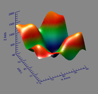 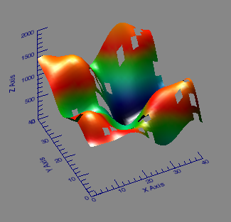 |
| On the left the original two-dimensional data set, and on the right the surface with missing data shown as holes. |
To use GRID_TPS, we need vectors that describe the good XY locations and the value of the surface at those locations. We will use these locations and values to reconstruct or interpolate the missing values. Type the following commands to create the X, Y, and Z vectors we need.
    goodIndices = Where(Finite(missingPeak), count)
   xy = Array_Indices(dims, goodIndices, /DIMENSIONS)    x = Reform(xy[0,*])
   y = Reform(xy[1,*])    z = missingPeak[goodIndices]
The only thing left is to create a gridded surface with GRID_TPS, using these values. Our grid will be the size of the original grid, start at location [0,0] in X and Y, and will have a grid spacing of 1 in both X and Y directions. In other words, it will be a grid with the original dimensions.
   fittedSurface = GRID_TPS(x, y, z, NGRID=dims, START=[0,0], DELTA=[1,1])
   cgSurface, fittedSurface, /ELEVATION, /SHADED
You see in the figure below that the fitted surface looks almost identical to the original surface.
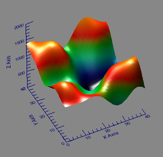 |
| The reconstructed surface looks almost identical to the original. |
But how close is it really? Type these commands to locate the bad indices and fix them. The difference between the corrected data and the original data is small.
   badIndices = Where(Finite(missingPeak) EQ 0)    correctedPeak = missingPeak
   correctedPeak[badIndices] = fittedSurface[badIndices]
   difference = peak - correctedPeak
   Print, 'Min/Max Difference from Orginal: ', Min(difference), Max(difference)
        Min/Max Difference from Orginal:      -2.58771      2.6143
In fact, the error is a very small percentage of the total data range.
    Print, 'Maximum Percent Difference: ', Max(Abs(difference)) / (Max(peak)-Min(peak)) * 100.0
      Maximum Percent Difference:      0.168670
The small percentage error gives confidence that thin plate splines might be an appropriate technique for data correction in this instance.
Note, that if you wanted to use the MIN_CURVE_SURF function to create a surface with a minimum curvature, you could execute this code. The MIN_CURVE_SURF function takes quite a bit longer to execute and should only be used with small areas.
fittedSurface = Min_Curve_Surf(z, x, y, GS=[1,1], BOUNDS=[0,0,40,40], NX=41, NY=41)
![]()
Version of IDL used to prepare this article: IDL 7.1.2
![]()
Copyright © 2009 David W. Fanning
Last Updated 29 December 2009