
TOMS Aerosol Display Program
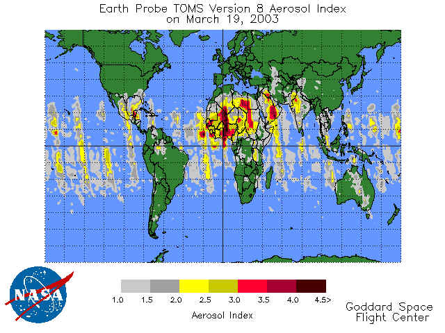
QUESTION: I am having a great deal of difficulty getting the TOMS aerosol data I downloaded from the NASA TOMS data center to look like the picture of the TOMS data on the NASA web page. I can get it on some kind of map projection, but I can't figure out how to get the oceans colored blue and the continents colored green, with the image data over the top of that. And what I produce in my PostScript file doesn't look anything like what I see on my graphics display. Help! Here is what the NASA image looks like.
 |
| This is what the user would like to be able to reproduce in IDL. |
Moreover, I would like to be able to zoom into just the African continent for my display. Here is what I have come up with so far (this is from my PostScript file). I can't see the continental outlines, the colors are wrong, and I haven't the foggiest idea how to color the oceans and landmass. Do you have any suggestions?
 |
| This is the user's first attempt at replicating the NASA image. |
![]()
ANSWER: As this is exactly the kind of question likely to show up in my morning e-mail, and as it involves (on my part) several hours of hard work, I've decided to answer it once and for all by writing a tutorial for how such a thing is accomplished. It is a good example, because there are several places where the gotchas can jump out and grab you by the throat, and because it can be exceedingly difficult to learn how to write device-independent graphics display programs by reading the IDL documentation. Plus, you are sure to learn a new technique or two for your IDL bag of tricks.
If you wish to run the code, you will need Coyote Library programs to do so. I don't know which ones. Lots of them, probably.
Obtaining the TOMS Data Set
The first order of business is to obtain the TOMS data set. I went to the NASA TOMS data center and requested the TOMS aerosol data for 19 March 2003. The data is returned in an ASCII text file. I opened the file in a text editor, because I didn't immediately know how to read it. The first three lines of the data file are these:
 Day:  78 Mar 19, 2003    EP/TOMS    NRT 360 RES  GEN:04.117 V8 ALECT: 12:00 AM
 Longitudes:  288 bins centered on 179.375 W to 179.375 E  (1.25 degree steps)
 Latitudes :  180 bins centered on  89.5   S to  89.5   N  (1.00 degree steps)
Thus, I learned that the data is in an array of 288 columns (longitude) by 180 rows (latitude), and I know the extent of the coverage (the entire Earth). By examining the rest of the data in the file, I learned that the data is stored in the file row by row, with each row containing 288 values packed into the file as three digit integers. Oddly, the 288 values in each row seemed to be packed 25 to a data file row, with the last data file row containing the last 13 values and a string giving the latitude of the row. This string threw me off a bit, and required a different approach to reading the data then I had planned.
I learned by poking around the TOMS web page a little longer that these three digit integers should be divided by 10.0 to obtain the actual data value, and that the value 999 represented missing data in the data set. From examining the NASA picture, I assumed (incorrectly, as it turned out) that the data would range in value from 1.0 to something greater than 4.5. In fact, the data ranged from 0.0 to 5.4, with over 27,000 values less than 1.0.
Writing the Program
The requirements for the program were that the output appear the same on the display and in a PostScript file (impossible, but I assumed he meant nearly the same), and that the user be able to zoom into a portion of the data set. Since I heard no talk about widgets, I assumed he didn't mean “interactively zoom,” although now I think about it this would be an excellent exercise for the student to extend the program in this way.
Since we are talking about displaying the TOMS data on a map projection, zooming in immediately causes me to think of the LIMIT keyword to the Map_Set command. That seems natural and we will go with that.
I reasoned, further, that the user might want to get the data and the header information out of the program, so I thought I might provide output keywords for that purpose. And, finally, the user will want to select PostScript output by setting a PostScript flag. I called the program READ_TOMS_AEROSOL and I defined the procedure definition line as below. All arguments and keywords are optional. If a file name is not provided, the user will be prompted to provide a file name. Note that in defining keywords, the name of the keyword is on the left and the variable that holds the value of the keyword is on the right. Since I can't keep two definitions in my mind concurrently any better than you can, I give them both the same name. IDL knows what I am talking about, even when I don't.
PRO Read_TOMS_Aerosol, filename, DATA=data, HEADER=header, LIMIT=limit, PS=ps
I'd like you to think that I write my programs in the logical, well thought-out style I'm about to use to present this program to you. But if you have ever written a program in your life, you know what I am about to tell you is a lie. Most programs start out with the program definition statement, but beyond that programs evolve in a herky-jerky fashion that is best lumped together with sausage making and other pursuits it is best not to know too much about. Suffice it to say, if there is structure to a program it is usually imposed after the fact and after we know quite a bit more about the problem then we do when we start. (Of course, government programmers spend six months writing the program specs, so they don't have this organizational problem. Their problem is motivation and ennui from not living life dangerously.)
Error Handling
In any case, stuff happens, so we ought to plan for it. Thus, the error handling code. I prefer to Catch errors because it gives me more flexibility in handling them. Here is a very basic, and simple, Catch error handler. The only non-standard features are that it checks to see if a file unit is open and closes it if it is, and it checks to see if we have changed the color mode and restores it if we have. Note the cancelling of the Catch as the first line of the Catch error handler. This is to prevent infinite loops if you (Heaven forbid!) have a typo in your error handling code. The cgErrorMsg comand is a Coyote Library command. It will alert the user to the error by putting up an error dialog, and will print a nice traceback of the error in the user's Command Log window.
   Catch, theError
   IF theError NE 0 THEN BEGIN
      Catch, /Cancel
      void = cgErrorMsg()
      IF N_Elements(lun) NE 0 THEN Free_Lun, lun
      IF N_Elements(theState) NE 0 THEN Device, Decomposed=theState
      RETURN
   ENDIF
Opening the Data File
The next step is to open the data file. If the user hasn't supplied a file name, ask them to do so now. If they refuse, exit the program. Here is the code.
   IF N_Elements(filename) EQ 0 THEN BEGIN
      filename = Dialog_Pickfile(Filter='*.txt', Title='Select TOMS file for READING...')
      IF filename EQ "" THEN RETURN
   ENDIF
   OpenR, lun, filename, /Get_Lun
Note the use of the GET_LUN keyword, which obtains a logical file unit number out of a pool of numbers IDL manages and assigns it to the variable lun.
Reading the Data File
The next step is to read the data file. The first three lines in the file are header information. We read this into the header variable, which will permit it to be returned to the user if they call the program with the HEADER keyword and provide a named IDL variable to receive the value.
   header = StrArr(3)
   READF, lun, header
The TOMS data is a 288 column by 180 integer array. The data is converted to the real floating point values by dividing by 10.0. Missing data, also known as NANs, are indicated in the data file with the value 999.
I had hoped to read the entire (288,180) array at once, but was thwarted in that pursuit by a string variable at the end of each row of data. Thus, I had to read the data row by row, ignoring the string on the end of the row. I also stumbled over a single blank character at the start of each line in the text file. These are the sorts of oddities you usually encounter when you are reading a new data set for the first time. In my case, I had to add a breakpoint to the program and stop it near the point where I was reading the data and play around with the data interactively before I got things right. (I was rewinding the data file with the Point_Lun command.) In any case, I eventually discovered that the following code read the data correctly.
   data = IntArr(288, 180)
   line = IntArr(288)
   FOR j=0,179 DO BEGIN
      READF, lun, line, Format='(1x,25I3)'
      data[0,j] = line
   ENDFOR
   Free_Lun, lun
Handling Missing Data
The next step is to handle the missing data. I need to find the missing data values, represented as 999 in the integer data set, before I convert the data to floating point values by dividing by 10.0 to get the real data values. I use the Where function to locate the missing data locations or indices in the data array.
indices = Where(data EQ 999, count)
Once I have the missing data locations, I can convert the data to real values, and convert the missing data to NANs.
   data = data / 10.0
   IF count GT 0 THEN data[indices] = !Values.F_NAN
Note that the data values here will go back to the user in the DATA keyword.
Using Limits to Subset the Data
The header information, shown above, allows us to construct latitude and longitude vectors for the gridded data set. (We would have to do this if we wanted to contour the aerosol data on the map projection, for example, but we use it here for a different purpose.) The vectors are easily created with the cgScaleVector command from the Coyote Library.
   lat = cgScaleVector(Findgen(180), -89.5, 89.5)
   lon = cgScaleVector(Findgen(288), -179.375, 179.375)
We use the vectors in this example to locate the proper subsetting index number to use in subsetting the 2D data array. We use the IDL routine Value_Locate to identify those index numbers in the lat and lon arrays that correspond to particular LIMIT values. If the LIMIT keyword is undefined (the keyword wasn't used), the the subscript values are just those at either end of the two vectors. The code looks like this.
   IF N_Elements(limit) EQ 0 THEN BEGIN
      latsubs = [0,179]
      lonsubs = [0,287]
   ENDIF ELSE BEGIN
      IF N_Elements(limit) NE 4 THEN $
         Message, 'Usage: LIMIT=[latmin, lonmin, latmax, lonmax].'
      latsubs = Value_Locate(lat, [limit[0],limit[2]])
      lonsubs = Value_Locate(lon, [limit[1],limit[3]])
   ENDELSE
The data is subscripted like this.
   lat_sub = lat[latsubs[0]:latsubs[1]]
   lon_sub = lon[lonsubs[0]:lonsubs[1]]
   data_sub = data[lonsubs[0]:lonsubs[1], latsubs[0]:latsubs[1]]
Preparing the TOMS Data for Display
The next step is to prepare the TOMS data for display. A quick look at the NASA picture suggests the data be scaled between 1 and 4.5 in units of 0.5. There are seven colors to be displayed. Originally, I scaled the entire data set by setting the MIN and MAX keywords on BytScl to 0 and 4.5, respectively. But when I looked at the color display, it was different from the NASA picture. Then I realized that NASA was probably treating all values below 1.0 as background pixels. I was setting all those pixels to 1.0 before I performed the scaling. (This is the meaning of the MIN keyword.) Thus, I was overrepresenting values in the 1.0 to 1.5 aerosol index category. Eventually, I realized there were over 27,000 pixels with values less than 1.0, so this was a big error. I decided to scale the data the same way I was before, but this time I was going to keep track of the locations of those pixels with values between 0.0 and 1.0, and I was going to set those pixels to the background later in the process. The NAN pixels are also going to be set to the background, so I also need to keep track of those. First, I scaled the data into seven colors.
img = BytScl(data_sub, Min=1, Max=4.5, Top=6, /NAN) + 1B
Note I have added 1 to the result, so that the TOMS data is now scaled from 1 to 7, instead of from 0 to 6. I have learned from hard experience that if you are working with colors in a PostScript file, you want to stay well away from color indices 0 and 255. Use any other color indices, but not either one of those! (This is not bad advice, in general, as it turns out.)
I have arbitrarily decided to use color index number 10 for the “background” pixels. So I set the NAN pixels and the less-than-one pixels to this color index.
   indices = Where(Finite(data_sub) EQ 0, count)
   IF count GT 0 THEN img[indices] = 10

   lessThanOne = Where(data_sub LT 1.0, ltcount)
   IF ltcount GT 0 THEN img[lessThanOne] = 10
Note the way I “find” the NAN pixels. I can't find them as numbers, since they aren't numbers. I have to determine with Finite that they are not numbers.
Load the Drawing Colors
The next step is to load the program color tables for displaying the image data. Because I am trying to get similar results in PostScript, which is an 8-bit display device, I do not want to use 24-bit colors. I choose to work in the Color Index Mode, which allows me to specify colors as indices to the color table. But I don't want to change the color mode to Index Mode permanently, since I almost always want to be in True-Color Mode for most work in IDL. So I will save the current color mode so I can restore it before I exit the program. The color mode is also restored in the Catch error handler if I exit the program unexpectedly.
Device, Decomposed=0, Get_Decomposed=theState
I now load the colors I intend to use in the program. Notice that I start with a gray-scale color table. This is not requried, but it makes me feel safe. If something goes wrong I am not going to be mislead by strange colors. I use FSC_Color from the Coyote Library to load the colors. I do this primarily because I can load colors “by name,” and thus I can easily tell which colors I have loaded.
   LoadCT, 0, /Silent

   ; Aerosol index colors, loaded at indices 1-7.
   TVLCT, cgColor(['LIGHT GRAY', 'DARK GRAY', 'YELLOW', 'GREEN YELLOW', $
                     'RED', 'MAROON', 'DARK RED'], /Triple), 1
   TVLCT, cgColor('BLACK', /Triple), 8 ; Drawing color.
   TVLCT, cgColor('SKY BLUE', /Triple), 250 ; Ocean color.
   TVLCT, cgColor('FOREST GREEN', /Triple), 251 ; Landmass color.
   TVLCT, cgColor('WHITE', /Triple), 252 ; "Missing" color.
Note the use of color index 252 as the “missing” color index. A missing color is a color that is not really a part of the plot. You could think of it as the background of the plot itself. In an graphics window it is normally black, although in PostScript is is normally white. Since I want the display to look the same as it does in PostScript, I chose white as the missing color, but assign the color to a color index other than 0 or 255.
Creating a Background Image in the Z-Graphics Buffer
If there is a clever part of the code, this is it. I need to make a background image of the world, with the oceans colored in blue, and the continents colored in green. Presumably to make such an image I need a landmask image and a seamask image. IDL does not offer such a thing automatically. It has to be created. That is what I am doing in this part of the code.
I am going to make the image in the Z-graphics buffer. Not because I have to, but because it is convenient. In the original version of this program I made the background image in the graphics window that was already open on the display. That is a good solution, too, but not as portable. After all, the user might not want to see a graphics window. Perhaps they just need a PostScript file, or perhaps they are running IDL remotely and don't have a graphics display. The Z-graphics buffer is a window that is rendered in software, so it is convenient for creating a window when you don't really want a window, if you know what I mean.
To do this properly, the image I want has to be a particular size. This is a problem because images (as well as “windows”) are sized differently in PostScript than they are on the graphics display. I have to use some IDL kung-fu to get what I want. First, I've decided to set my window size in pixel units. If I am trying to get PostScript output, I will divide these values by 100 and treat them as inches! Hai-ya! You will see how this works in a minute. For now, allow me to get my Z-graphics buffer set up. Notice I erase the buffer to be sure there is nothing left inside it when I want to use it.
   x_winsize = 750
   y_winsize = 600
   thisDevice = !D.Name
   Set_Plot, 'Z'
   Erase
   Device, Set_Resolution=[x_winsize, y_winsize], Z_Buffer=0
Notice how I save the name of the current graphics device. This is an essential technique for writing portable IDL code. The colors I loaded previously are copied into the Z-graphics buffer when I issue the Set_Plot command, but I could also use the COPY keyword to be sure.
The next step is to create a map projection and use Map_Continents to produce a landmass image. I am going to use Map_Set to create the map projection because it is easy and because the NASA image looks like it uses a common cylindrical map projection. To create a map projection that works everywhere (and I mean, in particular, across the International data line) I need to determine the center of the map limits. Here is my code. Notice I postition the map projection in the window with the Position keyword so I have room to add a color bar later.
   ; Set up the map projection center coordinates.
   lat_center = (Max(lat_sub) - Min(lat_sub)) / 2 + Min(lat_sub)
   lon_center = (Max(lon_sub) - Min(lon_sub)) / 2 + Min(lon_sub)

   ; Set up the map projection coordinate space, and draw the continents in a filled color.
   Map_Set, /Cylindrical, lat_center, lon_center, Position=[0.1, 0.25, 0.9, 0.9], $
      Limit=[Min(lat_sub), Min(lon_sub), Max(lat_sub), Max(lon_sub)], /NoBorder, /Isotropic
   Map_Continents, /Fill, Color=251
If I took a snapshot of the Z-graphics buffer right now, I would see something like what you see in the image below.
 |
| The landmask image in the Z-graphics buffer. |
If I capture this image properly, the pixels with values greater than 0 will be land pixels, and the values that equal 0 with be sea pixels. But before I can capture the image properly, I have to know what pixels to capture out of the entire window. The pixels I am interested in are the pixels behind the TOMS image.
Behind!? You haven't even put the TOMS image in the scene yet!
Whoops! That's right. And I don't want to put it in the scene yet, either, or I couldn't recover the right background pixels. I just want to know where the TOMS image would go if I did put it in the scene.
Humm. How can I figure out where it would go?
I could actually warp the TOMS image into the map projection space, and ask the Map_Image command to tell me where to place the image. It does this with the variables xx and yy. I can easily determine the size of the warped image. Those are exactly the coordinates I need to know if I want to capture the right portion of the window for my landmask and seamak images. Here is the code.
   warp = Map_Image(img, xx, yy, xs, ys, LatMin=Min(lat_sub), LonMin=Min(lon_sub), $
      LatMax=Max(lat_sub), LonMax=Max(lon_sub), Compress=1, Missing=252)

   ; Determine the size of the warped image.
   dims = Size(warp, /Dimensions)

   ; Grab this portion of the window to obtain sea and land mask images.
   snap = TVRD(xx, yy, dims[0], dims[1])
   seamask = snap EQ 0
   landmask = snap NE 0
   seacolor = 250
   seaimage = seamask * (BytArr(dims[0],dims[1]) + seacolor)
   landcolor = 251
   landimage = landmask * (BytArr(dims[0],dims[1]) + landcolor)
Notice I set the MISSING keyword in the Map_Image command to my “missing” color. This is critical. If I fail to do this I will have extremely strange results in my PostScript file.
Now I can create my background image and go back to my normal display device.
   backgroundImage = seaimage > landimage
   Set_Plot, thisDevice
If I took a snapshot of the background image now, it would look like this.
 |
| The background image in the Z-graphics buffer. |
Now, all I need to do is set the background indices in my warped image (remember, these have a value of 10) to the pixel values of the real background image.
   indices = Where(warp EQ 10, count)
   IF count GT 0 THEN warp[indices] = backgroundImage[indices]
Setting Up the Display Window
The next step is to set up the appropriate display window. This will either be a window on the display, or it will be a “window” in a PostScript file if the user set the PS keyword. Here is the code, then I'll explain what I am doing.
   IF Keyword_Set(PS) THEN BEGIN
      ps_xsize = x_winsize/100
      ps_ysize = y_winsize/100
      keywords = PSConfig(Cancel=cancelled, XSize=ps_xsize, YSize=ps_ysize, $
         Inches=1, XOffset=(8.5 - ps_xsize)/2.0, YOffset=(11.0 - ps_ysize)/2.0, $
         Filename='aerosol.ps')

      ; If the user cancelled, then forget about it.
      IF cancelled THEN BEGIN
         Device, Decomposed=theState
         RETURN
      ENDIF

      thisDevice = !D.Name
      Set_Plot, 'PS', /Copy
      Device, _Extra=keywords

      void = Map_Image(i, xx, yy, xs, ys, LatMin=Min(lat_sub), LonMin=Min(lon_sub), $
         LatMax=Max(lat_sub), LonMax=Max(lon_sub))

   ENDIF ELSE BEGIN

      Window, /Free, Title='TOMS Aerosol Data Plot', XSize=x_winsize, YSize=y_winsize
      Erase, Color=252

   ENDELSE
If the user wants to draw on the display, life is easy. Just create the window and erase it with the “missing” color.
If the user wants PostScript output, the situation is slightly more complicated. I've already mentioned my trick of dividing the window size by 100 and turning the numbers into inches to size the PostScript window. This is more of a convenience than a requirement. I like PostScript output to be as similar as possible to what the user sees on the display. This means, at the very least, getting the window aspect ratios correct. But I don't count on it too much, and, in fact, I am allowing the user (with fsc_psconfig) to change things if they don't much care for how I've set things up for them.
When they are satisfied, they hit the Accept button, and I configure the PostScript device in exactly they way they specified. If they hit the Cancel button I exit their life as if nothing whatsoever has happened. The return value from fsc_psconfig is a structure of keywords. I pass it along to the PostScript device using keyword inheritance.
The next line in the code, in which I am warping the image again, is one I wish I didn't have to use. It is so inelegant! But I haven't yet figured out a way around it. I need image starting coordinates and image sizes to position the color bar (the variables xx, yy, xs, and ys), and these values are just calculated differently in PostScript than they are in other devices. Thus, I've had to use the Map_Image command again just to get these values right. Yuck! Maybe someone will have a solution for me.
Display the Graphics
Finally, we are ready to display the graphics. First, the warped image. We use the positioning and sizing variables to size and position the image in the display window. (The XSize and YSize keywords are not used on your graphics display. They are only for the PostScript output, but they do no harm and are used because we are writing device-independent code.)
TV, warp, xx, yy, XSize=xs, YSize=ys
Next, we add the continental and country outlines, and the grid lines. We do this now so they are drawn on top of the image and not visa versa.
   Map_Continents, Color=8
   Map_Continents, Color=8, Countries=1
   Map_Grid, Color=8
Lastly, we add the color bar. The color bar is positioned to fit just below the image. We don't know, exactly, where the image has been positioned, even though we originally used the POSITION keyword (in the Map_Set command) to position the map projection, because we also used the ISOTROPIC keyword that preserved the aspect ratio of the map projection. This often causes the image to be re-positioned inside the window. I've used cgcolorbar, a Coyote Library program, to display the color bar.
   ; Add a colorbar.
   xstart = Float(xx)/!D.X_Size
   xend = Float(xs)/!D.X_Size + xstart
   yend = Float(yy)/!D.Y_Size -  0.10
   ystart = yend - 0.075
   tickvalues = ['1.0', '1.5', '2.0', '2.5', '3.0', '3.5', '4.0', '4.5+']
   cgColorbar, NColors=7, Bottom=1, Range=[1.0, 4.5], Divisions=7, Format='(F3.1)', $
      Position=[xstart, ystart, xend, yend], XMinor=1, XTicklen=1, $
      Title='Aerosol Index', Font=0, Color=8, Ticknames=tickvalues
Cleaning Up
The final section of the code is just used to clean up. In particular, we must close the PostScript file (inserting the PostScript showpage command into the file so the page can be ejected from the printer), and change back to our normal graphics output device. The final task is to set the color mode back to what it was when we started the program.
   ; Finish.
   IF Keyword_Set(PS) THEN BEGIN
      Device, /Close_File
      Set_Plot, thisDevice
   ENDIF

   ; Restore system state.
   Device, Decomposed=theState

   END
Running the Program
To run the READ_TOMS_AEROSOL program, simply save the file as read_toms_aerosol.pro, compile it, and run it like this. Select the TOMS data file when prompted.
   IDL> .compile read_toms_aerosol
        Compiled module: READ_TOMS_AEROSOL.
   IDL> Read_TOMS_Aerosol
You should see output that looks similar to the image below.
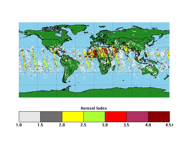 |
| The result of running the READ_TOMS_AEROSOL program. |
To zoom into the map project, use the LIMIT keyword. For example, to zoom into the African continent and Southern Europe, type this.
IDL> Read_TOMS_Aerosol, LIMIT=[-20, -20.5, 60, 72]
You should see output similar to the image below.
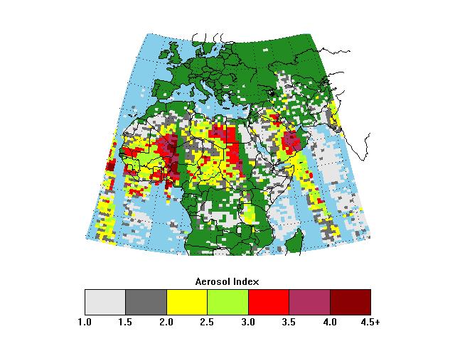 |
| The result of running the READ_TOMS_AEROSOL program with the LIMIT keyword. |
And, finally, try creating PostScript output. You will need a PostScript viewer to see the output. IDL> Read_TOMS_Aerosol, LIMIT=[-20, -20.5, 60, 72], /PS
![]()
Copyright © 2006 David W. Fanning
Last Updated 18 January 2006