
Analyzing Image ROIs
QUESTION: I have previously written about finding the boundary of a region of interest (ROI) or “blob” in an image, and fitting an ellipse to an image to give you some idea of the shape of the ROI. But in putting some of those ideas into practice the other day, I realized there was something I missed telling you. In fact, I didn't realize it myself. I wanted to put these ideas together in a slightly different way, and offer some software to do it, in this article.
![]()
ANSWER: The standard way of analyzing ROIs (I will call them “blobs” from now on) is to prepare a bi-level image of 0s and 1s, and use Label_Region to automatically identify the connected regions in the image and assign them a unique integer value. But, of course, Label_Region has problems with blobs on the boundaries of the image, so you have to prepare a special, slightly bigger, image to handle this before you do the analysis. That's kind of a pain in the neck.
And then, in one of the articles above, I suggest you find the indices of each blob by using a Where function on the image that is output from Label_Region. I've done this in the past, and it works fine. But in the past I have worked with relatively small images. The other day, I was working with big images, and this step turns out to be extremely slow. My program, in which I was trying to process about 11,000 blobs, took about 45 minutes to run! Completely unacceptable.
I wish I could tell you I found the answer by reading my own web page (the answer was there!), but alas I had to discover the answer empirically like everyone else. And the answer was, as you can probably guess if you have read many articles on this web page, a Histogram.
Specifically, it is (almost infinitely!) faster to take a Histogram of the output image from Label_Region and find the indices of individual blobs by using the reverse indices of the Histogram command than it is to use the Where function. My 45 minute program ran in 10 seconds after I made this change. In case you missed that, that is 270 times faster than it ran before. (Please don't tell me you have never heard of the Histogram function speeding up IDL code by factors of hundreds or thousands.)
Translated to IDL code, these ideas look like this.
    s = Size(biLevelImage, /DIMENSIONS)     fixLabelRegionImage = BytArr(s + 2)
    fixLabelRegionImage[1,1] = biLevelImage
    labelRegionOutput = Label_Region(fixLabelRegionImage)
    labelRegionOutput = labelRegionOutput[1:s[0], 1:s[1]]
    h = Histogram(labelRegionOutput, MIN=1, REVERSE_INDICES=ri, BINSIZE=1)
To find the indices of, say, the fourth blob (indexed as in all of IDL by a 3), you now simply do this.
indices4th = ri[ri[3]:ri[4]-1]
I've made all of this rigamarole significantly easier to do by packaging all these ideas up into an object named Blob_Analyzer. With this program, the code above is simplified to this.
   theBlobs = Obj_New('Blob_Analyzer', biLevelImage)
   indices4th = theBlobs -> GetIndices(3)
(Note that if you download Blob_Analyzer you will want to also download a new version of Fit_Ellipse, as it had to be changed to work more efficiently with the Blob_Analyzer program.)
Methods exist in this object to find out how many blobs Label_Region found, to return blob statistics, to fit ellipses to blobs, and to print statistical information on all the blobs found to the display or to a file. An example program exists in the file to show you one way Blob_Analyzer can be used. The results of running the example program are shown in the figure below.
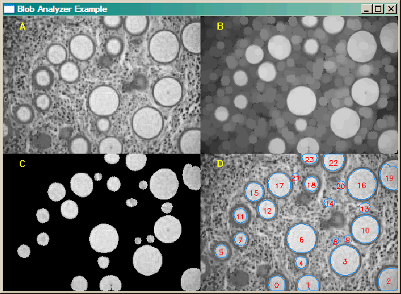 |
| (A) The original image. (B) The original image opened with MORPH_OPEN. (C) The bilevel input image to the Blob_Analyzer object. (D) The blobs identified by index number, with their perimeters displayed. |
Calling the ReportStats method on the object results in this output.
   IDL> theBlobs -> ReportStats
  INDEX   NUM_PIXELS   CENTER_X    CENTER_Y   PIXEL_AREA   PERIMETER_AREA   PERIMETER_LENGTH  MAJOR_AXIS   MINOR_AXIS    ANGLE
     0        426        107.89       9.78       106.50          98.00            37.56          12.15        11.29       -8.05
     1        580        151.97      10.22       145.00         134.25            49.21          17.49        11.77       -0.99
     2        812        266.29      15.36       203.00         190.75            52.56          17.88        14.65     -107.48
     3       1438        204.53      43.29       359.50         344.13            70.23          21.68        21.12      -76.47
     4        231        142.10      40.58        57.75          51.38            28.02           8.99         8.24      -69.08
     5        278         29.38      56.06        69.50          62.88            30.26           9.68         9.15      -73.57
     6       1391        142.79      74.15       347.75         332.50            69.11          21.11        20.99     -106.58
     7        261         56.45      73.29        65.25          58.75            29.56           9.45         8.82      -96.80
     8         81        191.00      71.00        20.25          16.50            16.49           5.10         5.10      -90.00
     9        100        208.64      73.64        25.00          20.88            18.19           5.80         5.52      -45.00
    10       1233        233.13      87.28       308.25         294.00            64.70          19.97        19.67     -114.43
    11        311         56.26     106.61        77.75          70.50            32.56          10.62         9.34      -76.65
    12        548         93.97     115.23       137.00         127.50            42.80          13.80        12.64      -72.87
    13        200        232.08     117.79        50.00          44.25            25.73           8.40         7.62       39.20
    14        155        181.97     125.07        38.75          33.50            23.31           8.48         6.10        1.01
    15        540         75.62     140.30       135.00         125.75            43.04          13.50        12.75      -89.02
    16       1441        227.93     151.28       360.25         344.75            70.53          22.37        20.52       82.17
    17        893        111.45     150.51       223.25         211.25            54.87          17.75        16.03      -66.11
    18        328        156.61     151.55        82.00          74.75            33.38          10.65         9.82      -85.27
    19        772        267.46     161.49       193.00         180.38            55.92          19.20        13.02      -74.79
    20        121        198.26     150.00        30.25          25.75            19.90           6.23         6.21     -270.00
    21        100        134.36     161.64        25.00          20.88            18.19           5.80         5.52     -135.00
    22        615        188.07     183.32       153.75         143.25            45.97          15.91        12.74        7.86
    23        270        154.14     187.57        67.50          60.50            30.73          12.79         7.72       -0.30
Many thanks to Ben Tupper for showing me an even more sophisticated version of this code that he wrote for his own analysis projects. I've stolen a couple of good ideas from him. Over time, and as I need them, I hope to incorporate more of those ideas into this program.
![]()
Version of IDL used to prepare this article: IDL 7.0.3.
![]()
Copyright © 2008 David W. Fanning
Last Updated 19 August 2008