Overlay Point Source Data on a Map

QUESTION: I have a carbon soil content dataset that I would like to overlay on a world map, like in the figure below. As far as I can tell, the data cannot be gridded into an image or into a 2D data set that I can contour. Instead, each data point is associated with a latitude and longitude coordinate. How can I display this point source data on a map in IDL?

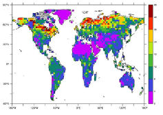This is what the figure should look like when finished.

ANSWER: The person asking this question supplied the data sets containing the soil carbon values, as well as the latitude and longitude values associated with these values. I have made them available as an IDL save file, named ptsource_carbon.sav. A complete example of this plot, along with the data, is available in the Coyote Plot Gallery. Restoring this file results in three variable, lat, lon, and soilc, each of which is a vector with 67420 elements.

   IDL> Restore, File='ptsource_carbon.sav'
   IDL> Help, lat, lon, soilc
        LAT             INT       = Array[67420]
        LON             INT       = Array[67420]
        SOILC           FLOAT     = Array[67420]

Perhaps the easiest way to do this is to use the indexed color model, so let's set that up and create a window to hold the graphics.

   IDL> SetDecomposedState, 0, Current=currentState
   IDL> cgDisplay, 600, 400, /Free, Title='Point Source Overlay on Map'

The next step is to set up the colors for the soil carbon values. A quick look at the figure provided by the user shows the carbon values differentiated by eight colors. I couldn't read the values on the color bar in the figure, but a quick look at some soil carbon web pages convinced me that the values were in tons per hectare. This could be wrong, but in the absence of other information, is probably a good enough guess for our purposes.

I picked colors that resembled the colors in the figure, and loaded them starting at color index 1. Remember to avoid color indices 0 and 255 if you want your programs to work in PostScript, too! I used, naturally, cgColor to select the colors, since I can do that in a natural way with color names.

   IDL> soil_colors = ['purple', 'dodger blue', 'dark green', 'lime green', $
          'green yellow', 'yellow', 'hot pink', 'crimson']
   IDL> TVLCT, cgColor(soil_colors, /Triple), 1

I have to scale the actual soil carbon values to use these colors, too, so I do that at the same time.

   IDL> soilc_colors = BytScl(soilc, Top=7) + 1B

A look at the figure provided by the user suggested a cylindrical map projection, but Antarctica is not shown. Thus, the latitude has been clipped at about -60 degrees. (Probably little soil carbon in Antarctica anyway!)

I also noticed that the figure uses a white background. There is no Background keyword for the cgMap_Set command, so to get a white background you have to erase the window with a white color, then use cgMap_Set with the NoErase keyword set. I also wanted to have room in the window for the color bar that I would add later. Thus, I set up my map projection space like this.

   IDL> cgErase
   IDL> cgMap_Set, /Cylindrical, /NoBorder, /NoErase, $
           Limit=[-60, -180, 90, 180], Position=[0.1, 0.1, 0.8, 0.9]

Initially, I just tried to plot the data directly at this point. Point source data is most easily plotted with the PlotS command, using the PSym keyword. But, I wanted to use a filled symbol of some sort and IDL doesn't provide a filled symbol in its (short) list of standard symbols. Of course, I could make my own filled symbol using the UserSym command, but it is much easier to just use one of the filled symbols from the cgSymCat program from the Coyote Library. I chose symbol number 15, a filled square symbol.

   IDL> symbol = cgSymCat(15)
   IDL> PlotS, lon, lat, PSym=symbol, Color=soilc_colors, SymSize=0.5

The final step is just to complete my display by adding continental outlines, a map grid, and a color bar, before switching back to the color model in place before I changed it.

   IDL> cgMap_Continents, Color='charcoal'
   IDL> cgMap_Grid, /Box, Color='charcoal'
   IDL> cgColorbar, /Vertical, Position=[0.87, 0.1, 0.9, 0.9], Bottom=1, NColors=8, $
           Divisions=8, Minor=0, YTicklen=1, Range=[0,Max(soilc)], AnnotateColor='charcoal', $
           /Right, Title='Ton/ha', Format='(F5.3)'
   IDL> SetDecomposedState, currentState

You see the results in the figure below. Note the rather large number of points that do not appear to be over land. These might be small islands, too small to be seen on a map of this resolution, or they might come from some other source, I don't know. They don't appear in the reference figure, and the user did not want them cluttering up the map, so they had to be removed.

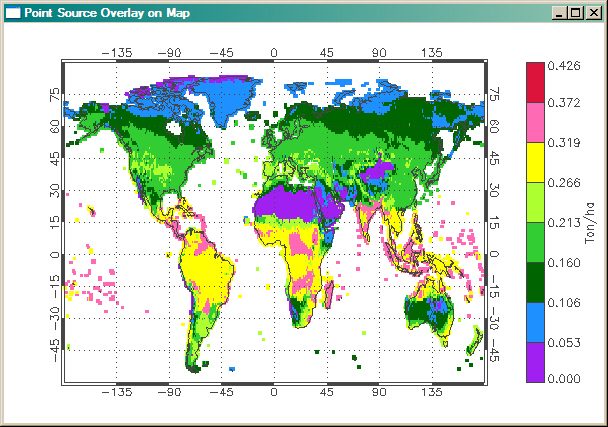First attempt at point source overlay on map.

The first attempt at drawing the point source overlay onto the map projection.

To decide if the overlay points were on "land" or not, I needed to create a land mask. With such a mask, I could screen out points that appeared on my map to be over water, thereby cleaning up the display.

It is possible to create a land mask with Map_Continents with the Fill keyword set. By taking a snapshot of the window with the continents filled in, I could obtain a land mask, but these would be in device or pixel coordinates. To check my overlay points, I have to convert the latitude and longitude coordinates from the data coordinate system to the device coordinate system. Fortunately, this is easy to do with the Convert_Coord command.

In the end, then, what I had to do was replace the PlotS command above with the following commands.

   IDL> cgMap_Continents, Color='black', /Fill
   IDL> mask = TVRD()
   IDL> dc = Convert_Coord(lon, lat, /Data, /To_Device)
   IDL> indices = Where(mask[dc[0,*],dc[1,*]] EQ 0)
   IDL> symbol = cgSymcat(15)
   IDL> PlotS, lon[indices], lat[indices], PSym=symbol, Color=soilc_colors[indices], SymSize=0.5

You can see the final result in the figure below. If you like, you can download the PointSourceOverlay program that contains the code for this example. Be sure you have the IDL save file ptsource_carbon.sav in the same directory as the program source code.

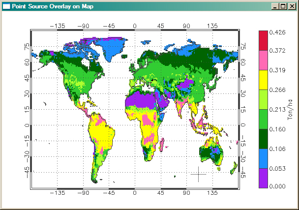The final display.