Coyote Graphics Plot Gallery
This is a gallery of example IDL programs and graphics plots, written using
Coyote Graphics routines. Its
purpose is to demonstrate the best programming practices for creating direct graphics graphical
output in IDL. Click any image to see a larger representation of the graphical output. You will
need to
install the Coyote Library to run these programs successfully.
Each example program consists of an IDL procedure that will create the graphical output in an IDL graphics
window. Following each program is a main-level IDL program that will run the example program and display
the graphical output in both a normal IDL graphics window and in a resizeable graphics window. In addition,
the main-level IDL program will create both a PostScript file and a PNG file of the graphical output.
PNG file output requires that ImageMagick
is installed properly on your machine. If this is not the case,
simply remove or comment out the last line in the main-level program before running the program.
If these programs don't run as you think they should, please
follow these steps to resolve
the problem. You will need a version of the
Coyote Library
that was created
on or after 14 January 2014 to run all the programs in the gallery.
Disclaimer for Function Graphics Code: For the most part
the function graphics code available on this page was made available to me by Matthew
Argall. I run the code (when possible) in IDL 8.2.3 and post the results. Your results
may differ from mine. I don't know what to tell you. I have a hard time, occasionally, getting
these programs to run correctly. For example, I just spent one and a half hours trying to
get Matthew's basic contour plot to display correctly on my machine and the contour labels were
still upside down. Later, we figured out how to right them. So, I'm just saying, use these function graphics routines
at your own risk. If you find a better way of doing things, we would love to hear it.

|
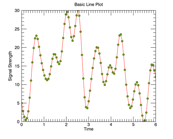
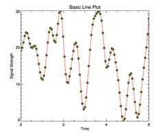
 Basic Line Plot
Additional Information
Basic Line Plot
Additional Information
|

|
|
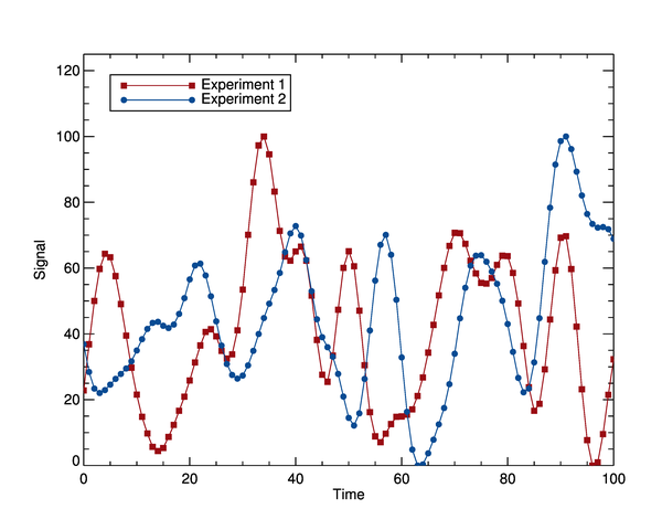
Line Plot with Legend
Additional Information
|
|
|
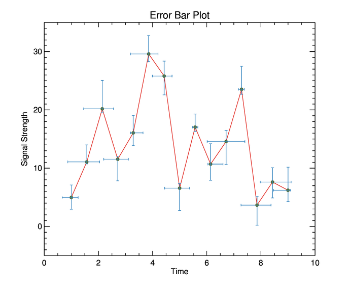
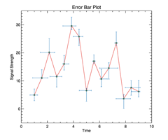
Error Bar Plot
Additional Information
|
|
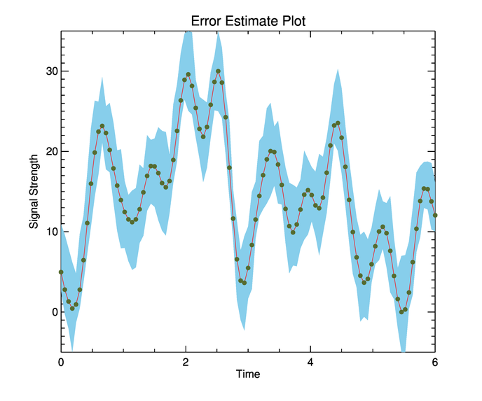
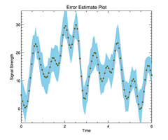
Error Estimate Plot
Additional Information
|
|
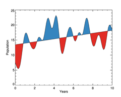
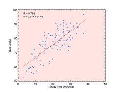
Linear Trend Plot
Additional Information
|
|
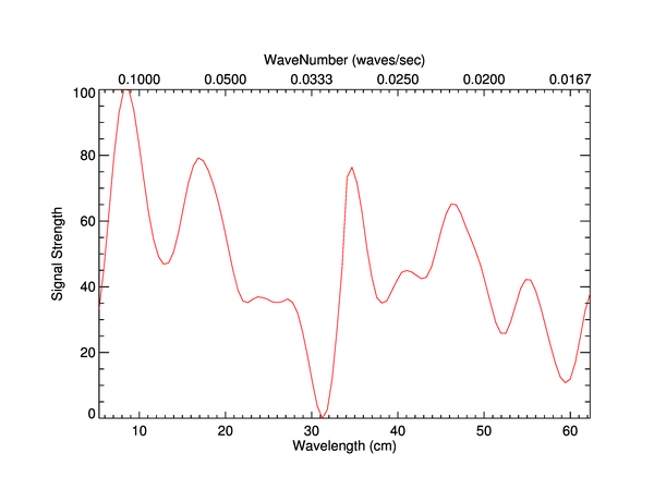
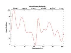
Wavenumber Plot
Additional Information
|
|
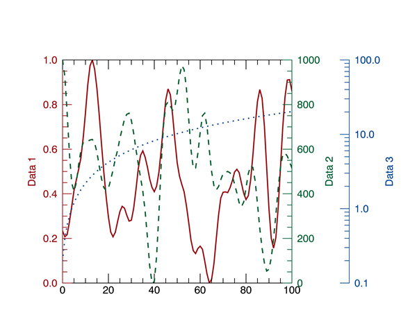
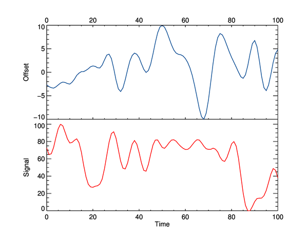
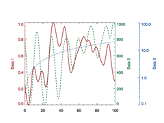
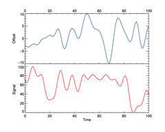
Additional Axes Plot
Additional Information
|

|
|
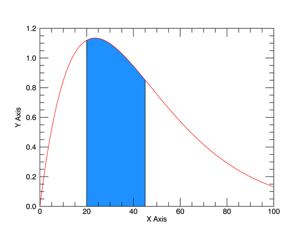
Filled Area Plot
Additional Information
|
|
|
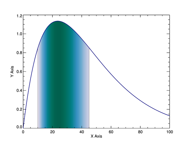
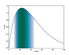
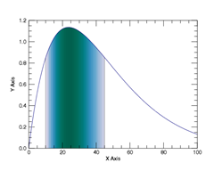
Filled Area Plot Colored by Height
Additional Information
|
|
|
Ladder Plot
Additional Information
|
|
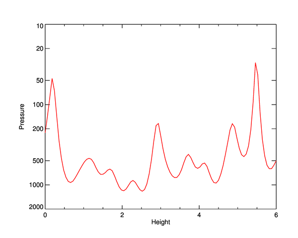
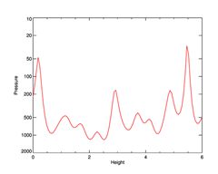
Logarithmic Pressure Plot
Additional Information
|

|
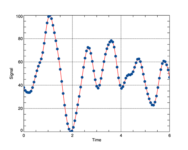
Grid on Line Plot
Additional Information
|
|
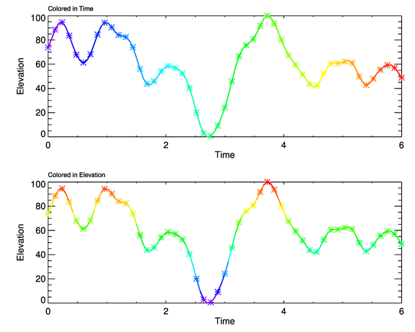
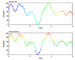
Colored Line Plots
Additional Information
|
|
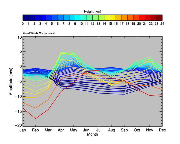
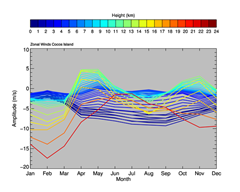
Zonal Wind Plot
Additional Information
|
|
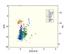
2D Scatter Plot
Additional Information
|
|
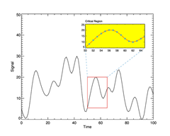
Plot Within a Plot
Additional Information
|
|
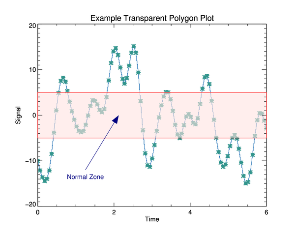
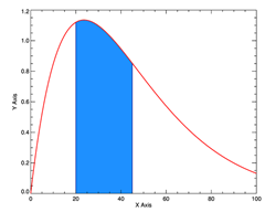
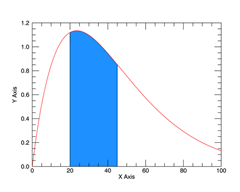
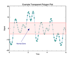
Transparent Polygon Plot
Additional Information
|
|
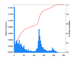
Histogram Plot with Cumulative Probability
Additional Information
|
|
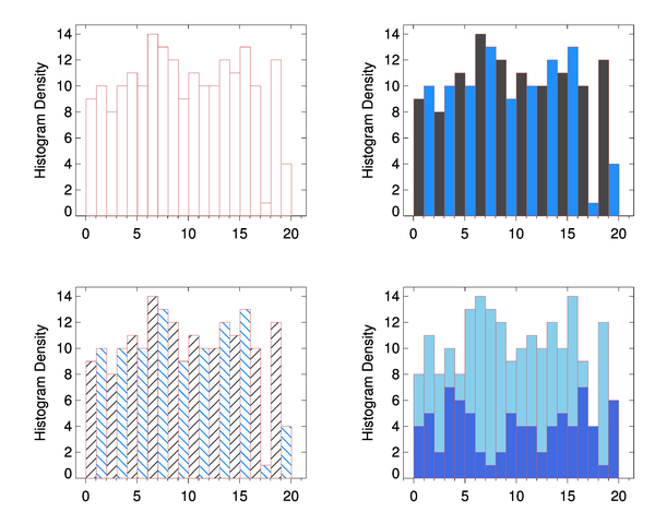
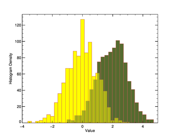
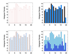
Various Histogram Plots
Additional Information
|

|
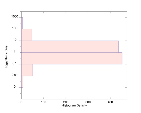
Rotated Histogram Plot with Logarithmic Bins
Additional Information
|
|
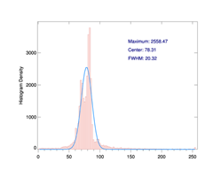
Fitted Gaussian Plot
Additional Information
|
|
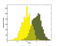
Transparent Histogram Plot
Additional Information
|
|
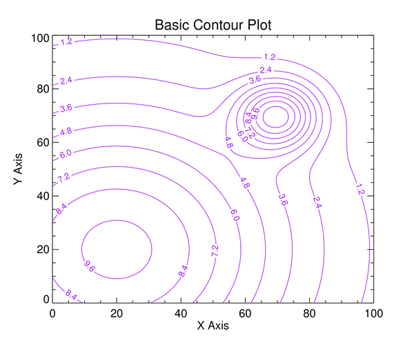
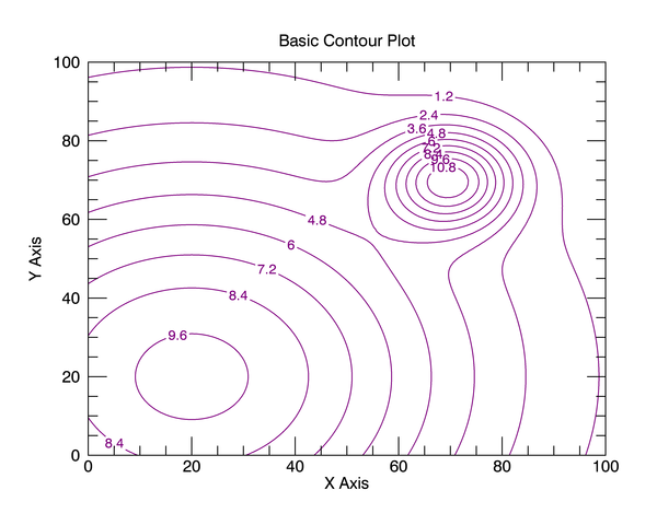
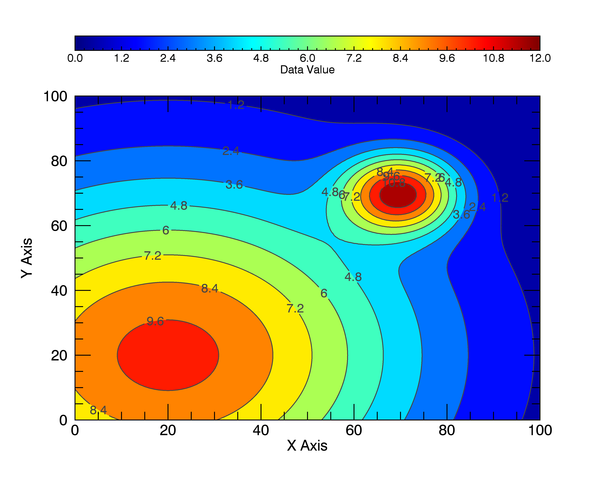
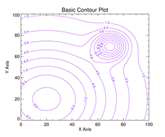
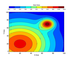
Basic Contour Plot
Additional Information
|

|
|
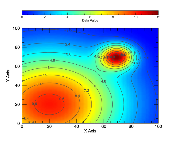
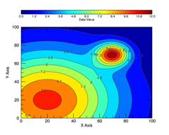
Filled Contour Plot
Additional Information
|
|

|
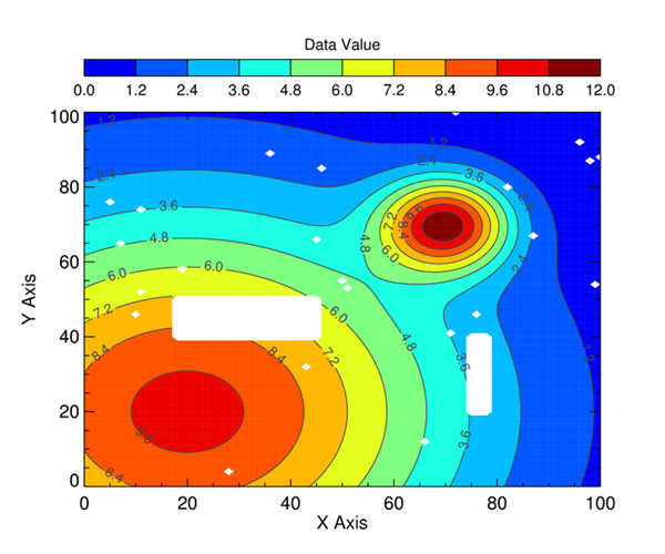
Filled Contour Plot with Missing Data
Additional Information
|
|
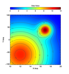
Image Plot with Contours Overlaid
Additional Information
|

|
|
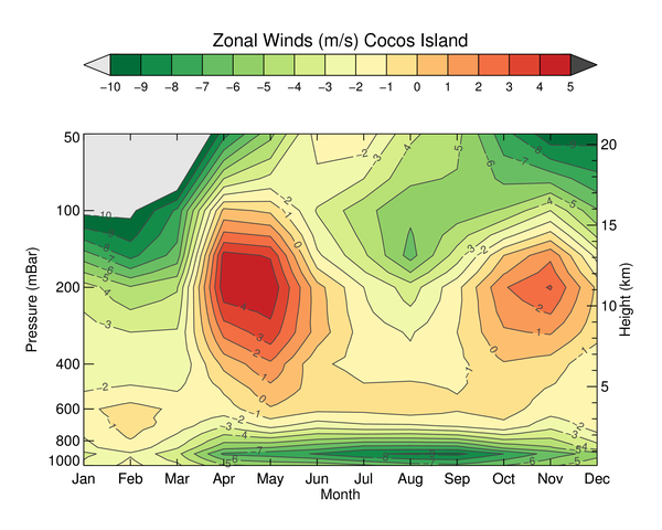
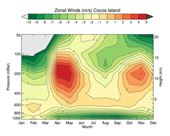
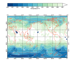
Zonal Wind Contour Plot
Additional Information
|
|
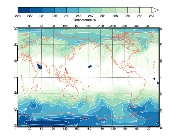
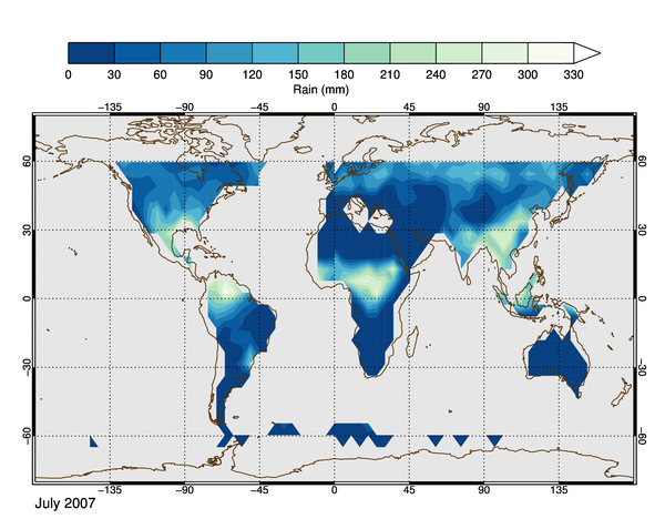
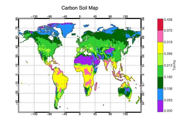
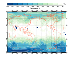
Filled Contours on a Global Map Projection
Additional Information
|
|
|
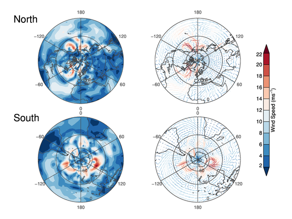
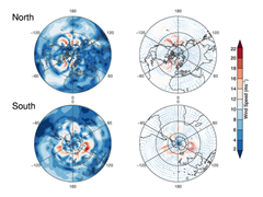
Polar Wind Filled Contour and Vector Plots
Additional Information
|

|
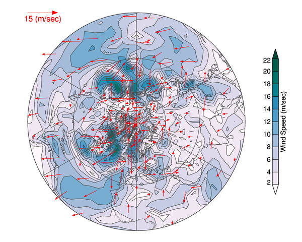
Velocity Vector Plots
Additional Information
|
|
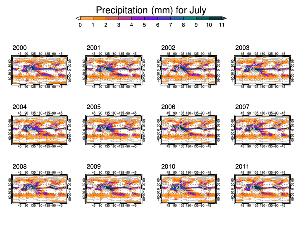
Small Contour Multiples Plot
Additional Information
|
|
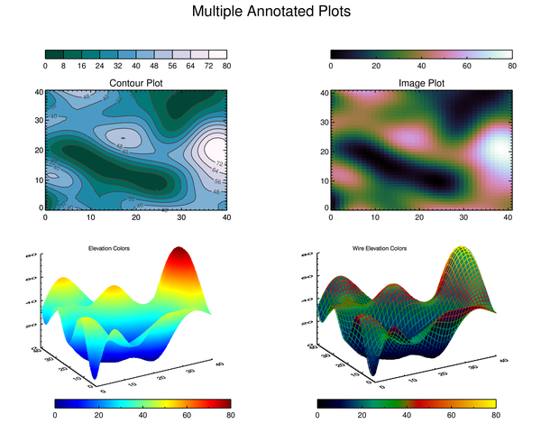
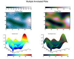
Multiple Plots with Annotations
Additional Information
|

|
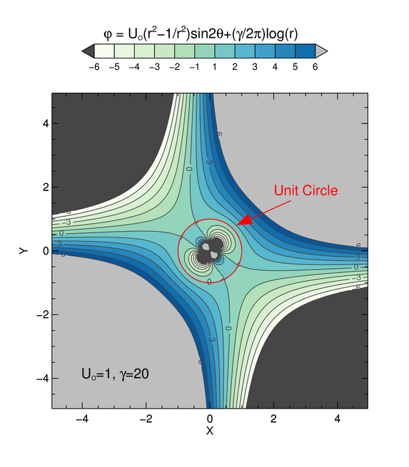
StreamFunction Plot with Greek Symbols
Additional Information
|
|
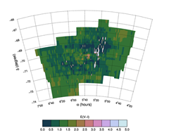
Curvilinear Extinction Map Plot
Additional Information
|
|
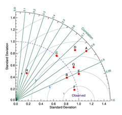
Taylor Diagram
Additional Information
|
|
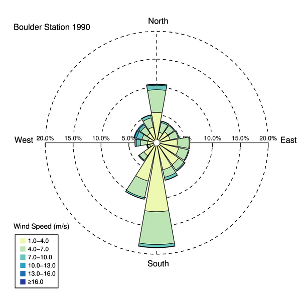
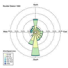
Wind Rose Plot
Additional Information
|
|
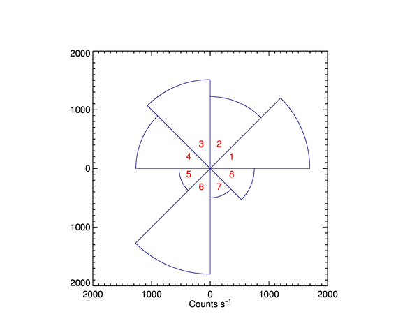
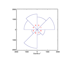
Anisotropy Pie Plot
Additional Information
|
|
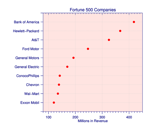
Dot Plot
Additional Information
|

|
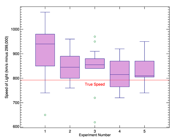
Box and Whisker Plot
Additional Information
|
|
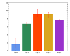
Bar Plot with Error Bars
Additional Information
|
|
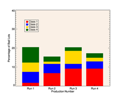
Overlapping Bar Plot
Additional Information
|
|
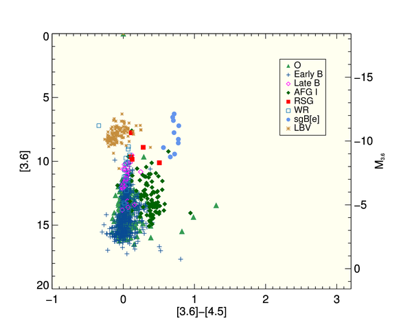
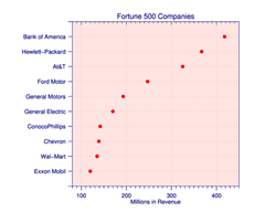
Symbol Plot with Legend
Additional Information
|
|
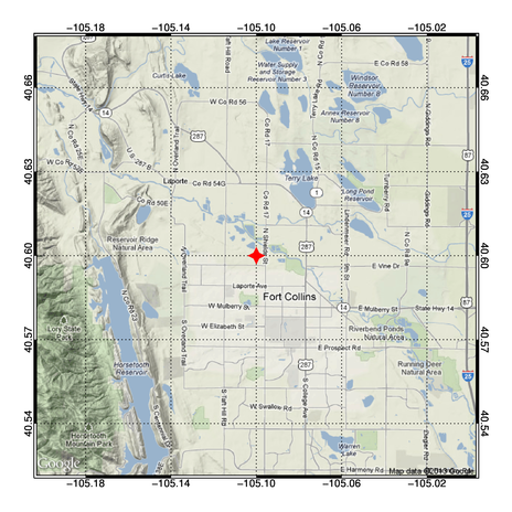
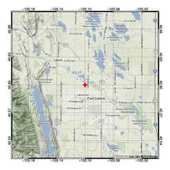
Google Map Plot
Additional Information
|
|
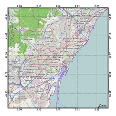
OpenStreetMap Plot
Additional Information
|
|
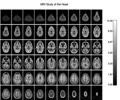
Multiple Image Plot
Additional Information
|

|
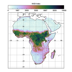
HDF-EOS Grid Plot
Additional Information
|

|
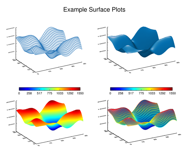
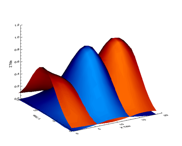
Surface Plots
Additional Information
|
|
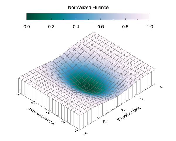
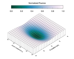
Fluence Surface Plot
Additional Information
|
|
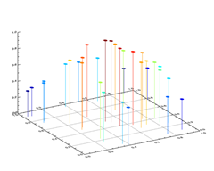
3D Scatter Plot
Additional Information
|
|
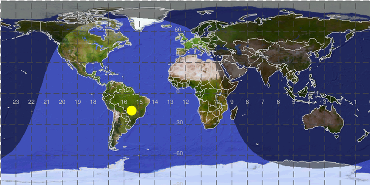
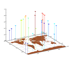
3D Scatter Plot on Map
Additional Information
|
|
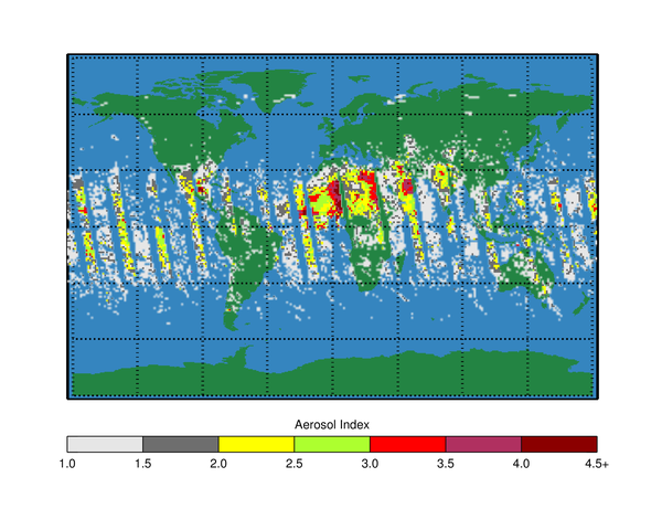
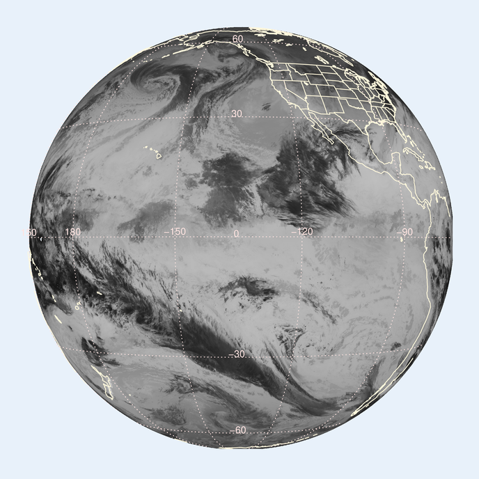
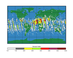
NASA TOMS Satellite Aerosol Plot
Additional Information
|
|
GeoTiff Registered Image Plot
Additional Information
|

|
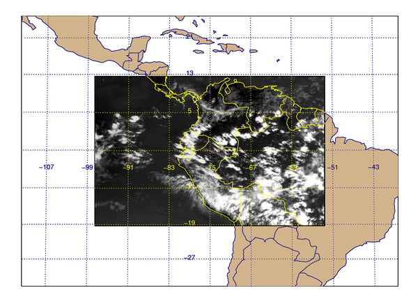
GOES Image Plot with Associated Lat/Lon Pixel Values
Additional Information
|
|
GOES GeoTiff Image Plot
Additional Information
|

|
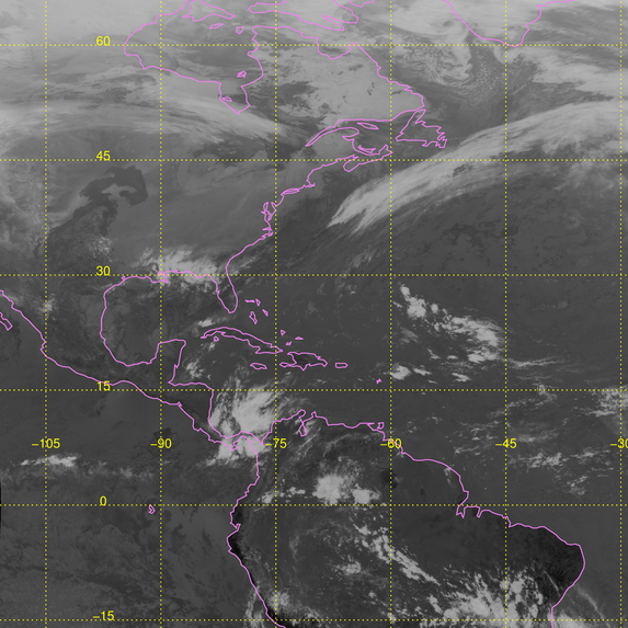
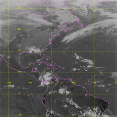
GOES-15 Geostationary Image Plot
Additional Information
|
|
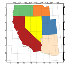
Shapefile Plot
Additional Information
|
|
Transparent Polygon on Map Plot
Additional Information
|

|
GSHHS Database Plot
Additional Information
|

|
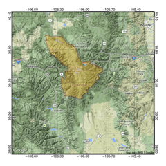
Overlay of Point Source Data on a Map
Additional Information
|
|
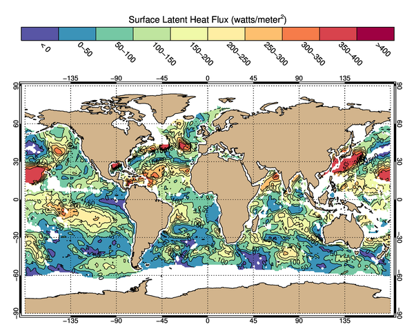
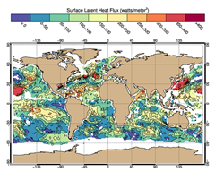
Latent Surface Heat Flux Plot from NASA HDF5 Data
Additional Information
|

|
Hidden Surface Plot
Additional Information
|
|
Isosurface Plot of 3D Data
Additional Information
|

|
Sun Terminator Plot
Additional Information
|
|
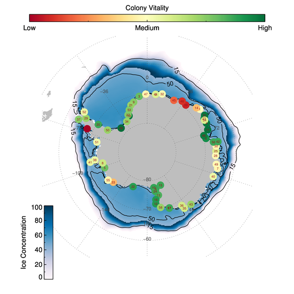
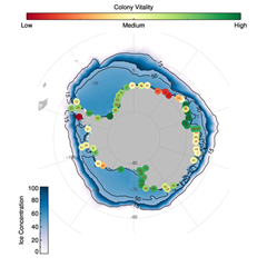
Penguin Colony Plot
Additional Information
|
|
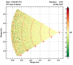
Lidar Range Plot
Additional Information
|

|
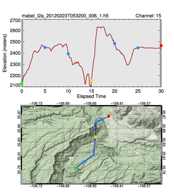
Lidar Track Plot with HDF5 Data
Additional Information
|
|
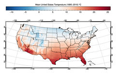
Mean US Temperature Plot with netCDF Data
Additional Information
|

|
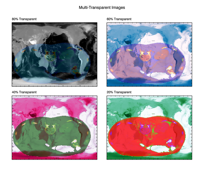
Multiple Transparent Images
Additional Information
|
|
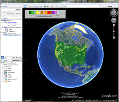
Preparing Data for Display on Google Earth
Additional Information
|
|
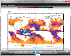
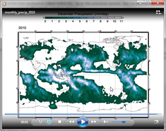
Creating an AVI Movie Animation
Additional Information
|
|
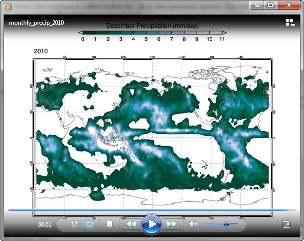
Creating an MPG-4 Movie Animation
Additional Information
|
Copyright © 2013 David W. Fanning
Written 27 January 2013
Updated 28 February 2014