Mapping Data Associated with Lat/Lon Arrays

QUESTION: I have data that is sometimes gridded and sometimes not. But, each data point is always associated with a latitude and longitude value. In the past I have used Map_Patch to display this kind of data. But, Map_Patch seems so 1970s. Do you have anything in your Coyote Graphics library that will do the job?

ANSWER: Yes, if you have data with associated latitude and longitude arrays, you want to grid that data for display with cgWarpToMap. This is the Coyote Graphics equivalent to Map_Patch.

To see how it works, copy the goes_example_data save file to a local directory. This file has been discussed previously in an article, entitled Navigating GOES Images. The procedure described here is much faster and more straightforward than the procedure described in that article.

To read and prepare the data, we type these commands.

    filename = 'goes_example_data.sav'
    Restore, filename
    peru_lat = Temporary(peru_lat) / 10000.
    peru_lon = Temporary(peru_lon) / 10000.
    Help, peruimage, peru_lat, peru_lon
         PERUIMAGE       BYTE      = Array[600, 431]
         PERU_LAT        FLOAT     = Array[600, 431]
         PERU_LON        FLOAT     = Array[600, 431]

We will need to know the center of this image of the map projection, so we find it like this.

    s = Size(peruimage, /DIMENSIONS)
    centerLat = peru_lat[s[0]/2, s[1]/2]
    centerLon = peru_lon[s[0]/2, s[1]/2]

The image is 600 by 431 in size, and the center latitude is -3.01190 degrees and the center longitude is -75.0101 degrees.

First, we will produce the same kind of output as was produced in the previous article so you can compare the two. We start, as before, by creating a map projection space. However, this time we use the Coyote Graphics routine cgMap, which among other things is a wrapper for Map_Proj_Init.

   mapPosition = [0.05, 0.05, 0.95, 0.95]
   map = Obj_New('cgMap', 'Albers Equal Area', Ellipsoid='sphere', $
         Position=mapPosition, Standard_Par1=-19, Standard_Par2=21, $
         Center_Lat=centerLat, Center_Lon=centerLon)

Next, we warp the data into a 2D grid that we will display. We will use a pixel resolution of 300 by 250 for the output image, which is fairly small. You can use any resolution you like, including resolutions that contain more pixels than the original image. We will also set the SetRange keyword, which will set the XRange and YRange properties of the map object internally, so we don't have to set these later, when we return from cgWarpToMap. The code looks like this.

   warped = cgWarpToMap(peruImage, peru_lon, peru_lat, Map=map, Missing=0, $
       Resolution=[300, 250], /SetRange)

Finally, we display the data.

    cgImage, warped, Stretch=2, Position=[0.1, 0.1, 0.9, 0.9], Background='white'
    map -> Draw
    annotateColor = 'Yellow'
    cgMap_Grid, Map=map, /Label, Color=annotateColor, /cgGrid
    cgMap_Continents, MAP=map, Color=annotateColor
    cgMap_Continents, MAP=map, Color=annotateColor, /Countries

You see the results in the figure below.

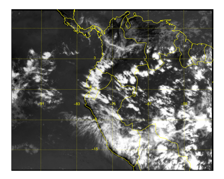The warped image created from data and associated latitude and longitude arrays.

 

If you would like to see more of the surrounding continents, to better place the map image in global space, you could do something like this. First, draw the larger map.

    map-> GetProperty, XRange=xrange, YRange=yrange
    map -> SetProperty, XRange=[xrange[0]-1.5e6, xrange[1]+1.5e6], $
           YRange=[yrange[0]-1.5e6, yrange[1]+1.5e6], /Draw
    cgMap_Continents, MAP=map, Color='tan', /Fill
    cgMap_Continents, MAP=map, Color='navy'
    cgMap_Continents, MAP=map, Color='navy', /Countries
    cgMap_Grid, Map=map, /Label, Color='navy', LATDEL=8, LONDEL=8, /cgGrid

Next, display the image, keeping track of the image position in the window. Using this information, update the map object, and draw map annotations just on the image, like this.

    cgImage, warped, Stretch=2, Position=mapPosition, OPosition=imagePos, $
         XRange=xrange, YRange=yrange, /Overplot
    map -> SetProperty, XRange=xrange, YRange=yrange, Position=imagePos
    annotateColor = 'Yellow'
    cgMap_Grid, Map=map, /Label, Color=annotateColor, LATDEL=8, LONDEL=8, /cgGrid
    cgMap_Continents, MAP=map, Color=annotateColor, /HiRes
    cgMap_Continents, MAP=map, Color=annotateColor, /Countries

You see the result in the figure below.

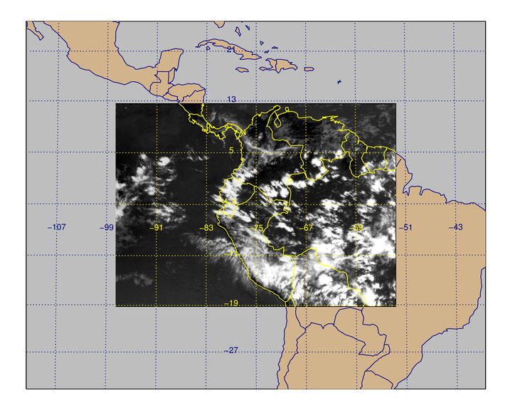The image displayed so more of its context is shown on the map.

 

All the commands used to create the graphics in this article can can be found here. As always, be sure you update your Coyote Library to the latest version of the files.

Version of IDL used to prepare this article: IDL 8.2.