
Comparing Graphics Output
QUESTION: I realize both Coyote Graphics and the new Function Graphics that was introduced in IDL 8 can produce various types of output files (EPS, PDF, PNG, JPEG, etc.), but I don't know how the output compares. Do you have any information on that?
![]()
ANSWER: Yes, I have done some tests to try to compare the two graphics systems. First, I've made sure that we are using the same size windows. The default window size for both systems is 640 in X and 512 in Y. So we are comparing the same thing, I have created the data and created a variable that will produce encapsulated PostScript, PDF, PNG, and JPEG files. I am using IDL 8.1 on a Windows 7 64-bit OS to produce the graphics output. I am providing the script I used to create the files described below. You can run the program to create the files yourself. You will need an updated Coyote Library to do so.
  data = cgDemoData(1)
  ext = ['.jpg', '.png', '.eps', '.pdf']
  numfiles = N_Elements(ext)
To create the Function Graphics output, I run this code.
  p = Plot(data, Position=[0.1, 0.1, 0.95, 0.85], $
     Color='red', Symbol='Circle', /Sym_Filled, $
     Sym_Color='blue', /Buffer, $
     Title='This is a Plot Title', $
     XTitle='Time in Seconds', $
     YTitle='Signal Strength')
  FOR j=0,numfiles-1 DO p.save, 'fg_plot_600dpi' + ext[j]
  p.close
To create the Coyote Graphics output, I first set the output parameters so that it uses 600 dpi scanning, and I run this code.
  cgWindow_SetDefs, IM_Density=600, IM_Resize=100
  FOR j=0,numfiles-1 DO $
     cgPlot, data, Position=[0.1, 0.1, 0.95, 0.85], $
        Color='red', PSym=-16, SymColor='blue', $
        Title='This is a Plot Title', XTitle='Time in Seconds', $
        YTitle='Signal Strength', Output='cg_plot_600dpi' + ext[j]
You see the results of running the code in the table below. The size of the output file is shown in KBytes, and the X size and Y size of the JPEG and PNG files are shown in pixels. In general, Coyote Graphics output is considerable smaller in file size, although the pixel dimensions are larger. I do not know how to explain this result. Right-clicking on the file size will allow you to download the file. Choose Save Link As... to save the file to disk. You can open these files in your browser, but I don't recommend it. They are so large, that they render poorly in a browser window. It is better to save the file to disk and open it with your usual raster file software. If you open the PDF files in your browser, be sure you view them at the same zoom factor. They open in my browser (Firefox) with different native "zooms". The Coyote Graphics file opens at 75%, and the Function Graphics file opens at 125%.
| Type of Output | EPS | PNG | JPEG | XSIZE | YSIZE | |
| Coyote Graphics | 42 | 25 | 161 | 773 | 5733 | 4583 |
| Function Graphics | 252 | 84 | 362 | 890 | 5339 | 4271 |
In general, the output is extremely similar, with the exception of the encapsulated PostScript files. The Function Graphics encapsulated PostScript file appears to be clipped off at the right-hand edge, at least when I open it in my GhostView PostScript viewer. But, I have turned each PostScript file into a PNG file, and show the results in the figures below. You can see that both encapsulated PostScript files create good PNG files (I used cgPS2Raster to create the files), which leads me to believe whatever is wrong with the encapsulated PostScript file from Function Graphics, it is not serious.
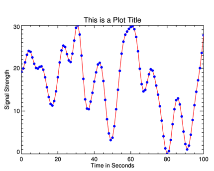 |
| The Coyote Graphics file is slighly smaller than the Function Graphics file. |
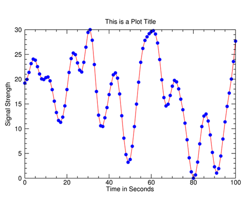 |
| The Function Graphics file looks similar to the Coyote Graphics file above it. |
I think it is exceedingly unlikely that you will be making many files at this resolution. Your colleagues will grow tired of your large e-mail attachments, certainly. I'm surprised this is the default resolution for Function Graphics. It seems more likely to me that you would want raster file output that was comparable in size to the graphics windows you are using.
We can create such files by simply modifying the code we used above. In the Function Graphics case, we just use the Resolution keyword on the Save method to select the resolution we want (300 and 75, in the tables below, although I am only providing results for the 75 dpi resolution for download).
    p.save, 'fg_300dpi' + ext[j], resolution=300
    p.save, 'fg_075dpi' + ext[j], resolution=75
In the Coyote Graphics case, we use the cgWindows_SetDefs procedure to set the resolution and resizing.
    cgWindow_SetDefs, IM_Density=300, IM_Resize=100
    cgWindow_SetDefs, IM_Density=300, IM_Resize=25
You see the results in the tables below. I've included the earlier table again so you can see all the results together.
| Type of Output | EPS | PNG | JPEG | XSIZE | YSIZE | |
| Coyote Graphics | 42 | 25 | 161 | 773 | 5733 | 4583 |
| Function Graphics | 252 | 84 | 362 | 890 | 5339 | 4271 |
| Type of Output | EPS | PNG | JPEG | XSIZE | YSIZE | |
| Coyote Graphics | 42 | 25 | 63 | 315 | 2867 | 2292 |
| Function Graphics | 252 | 83 | 158 | 336 | 2669 | 2135 |
| Type of Output | EPS | PNG | JPEG | XSIZE | YSIZE | |
| Coyote Graphics | 42 | 25 | 53 | 73 | 717 | 573 |
| Function Graphics | 252 | 54 | 33 | 81 | 667 | 534 |
The bottom line seems to be that the output is entirely comparable between the two graphics systems. I don't see much difference between them in terms of the quality of the output.
At the lowest resolution shown here, which is the default for Coyote Graphics, I think the Coyote Graphics output is slighly preferable, but I am not sure I have been completely fair to Function Graphics by setting the resolution so low. I was trying to produce a final result that had the right pixel size. There are obviously differences between what Function Graphics means by "resolution" and what Coyote Graphics means. I don't know, yet, how to resolve those differences.
![]()
Version of IDL used to prepare this article: IDL 8.1.
![]()
![]()


