
Gridding to the Surface of a Sphere


QUESTION: I have random data that are mapped to latitude and longitude values. I want to grid this data onto the surface of a sphere in order to display it as a contour plot on an orthographic map projection. I see that the Triangulate/Trigrid method of gridding data in IDL has this kind of spherical gridding functionality. But, the results are exceedingly strange!
The input data have values in the range 0 to 15. The output data, which I have gridded to the surface of a sphere, have values that range from -171 to 308. What in the world am I doing wrong?
   IDL> Triangulate, lons, lats, SPHERE=sTriangles, /DEGREES, FVALUE=data
   IDL> gridded = Trigrid(data, [0.5, 0.5], [0, -90, 360, 90], $
             SPHERE=sTriangles, XGRID=x, YGRID=y, /DEGREES)
   IDL> cgMinMax, data, Text='Original data values:'
        Original data values:  0.000000  14.4000
   IDL> cgMinMax, gridded, Text='Gridded data with Triangulate/Trigrid (Spherical) method.'
        Gridded data with Triangulate/Trigrid (Spherical) method. -171.51771  308.18993
![]()
ANSWER: I don't think you are doing anything wrong. I think the Triangulate/Trigrid method of gridding to the surface of a sphere just doesn't work correctly.
Allow me to illustrate what I mean with the data you sent me. I have created a program, SphericalGrid, which reads the data file and creates a series of data plots. I'll discuss these here.
The data you sent have these characteristics. I have named the variables lats, lons, and data.
   Latitude Range:        -87.2809      89.2679
   Longitude Range:      0.0886124      359.750
   Data Range:            0.000000      14.4000
To ensure we are comparing apples to apples, I am creating a contour plot with levels from 7.5 to 15, in units of 0.5. Values outside of this range are displayed with out-of-bounds colors. I set all this up with the following IDL commands.
   nlevels = 15
   cgLoadCT, 33, NColors=nlevels, Bottom=1
   TVLCT, cgColor('gray', /TRIPLE), 0              ; OOB low
   TVLCT, cgColor('charcoal', /TRIPLE), nlevels+1  ; OOB high
   c_colors = Bindgen(nlevels+1)
   levels = (Indgen(nlevels)+1) / 2.0 + 7
   levels = [0,levels]
Because you want to display this on an orthographic map projection, we will only be looking at half the data at any one time. To make this easy to understand, we will assume the orthographic projection is centered at 0 degrees latitude and 180 degrees longitude (assuming longitudes range from 0 to 360, as the data here does). This means we will be looking at the data that goes from 90 degress of longitude to 270 degrees of longitude.
To get a sense of what we are looking at, let's first just grid the data as if it were on a flat 2D surface, and display it as a filled contour plot on a normal cylindrical map projection. Here is the code. Note that I am not drawing the contour lines on the plot to keep the results as simple as possible.
   cgMap_Set, /Cylindrical, 0, 180, Position=[0.1, 0.1, 0.9, 0.8], Limit=[-90, 90, 90, 270]
   Triangulate, lons, lats, triangles
   gridded = Trigrid(lons, lats, data, triangles, [0.5,0.5], [0,-90,360,90], XGrid=x, YGrid=y)
   cgContour, gridded, x, y, Levels=levels, /CELL_FILL, C_COLORS=c_colors, /OVERPLOT
   cgMap_Grid, LatDel=20, LonDel=40, /Box_Axes
   cgColorbar, NColors=nlevels, OOB_Low=0b, Range=[7.5,15.0], Divisions=nlevels, $
       /Discrete, Format='(F0.1)', Bottom=1, OOB_High=Byte(nlevels+1), $
       Position=[0.1, 0.88, 0.9, 0.93]
You see the results in the figure below. In this example, the gridded data had a data range of 0.0000 to 14.2041, compared to the orginal data range of 0.0000 to 14.4000. This slight difference is what you would expect when the data is gridded.
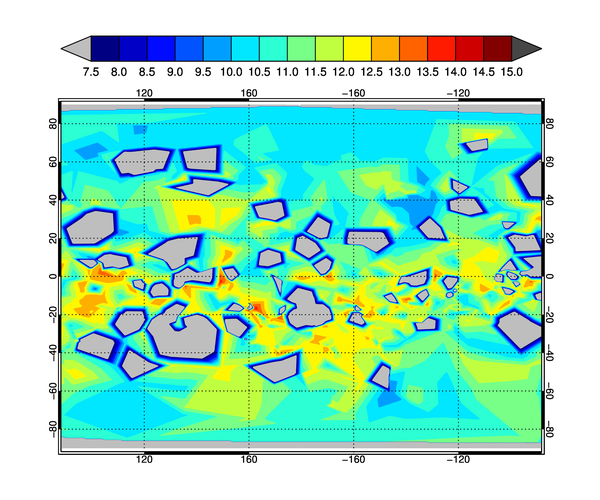 |
| The 2D gridded data displayed on a cylindrical map projection. |
![]()
Grid to Sphere Surface with Triangulate/Trigrid
Next, we use the Triangulate/Trigrid method to grid the data to the surface of a sphere and display that on an orthographic map projection. Here is the code. In this example, the data range of the gridded data is -171.5177 to 308.1899, values that simple must be wrong!
   Triangulate, lons, lats, tri, SPHERE=sTriangles, /DEGREES, FVALUE=data
   gridded = Trigrid(data, [0.5, 0.5], [0, -90, 360, 90], $
       SPHERE=sTriangles, XGRID=x, YGRID=y, /DEGREES)
   cgMap_Set, /ORTHOGRAPHIC, 0, 180, Position=[0.1, 0.1, 0.9, 0.8], /ISOTROPIC
   cgContour, gridded, x, y, /OVERPLOT, /CELL_FILL, C_COLORS=c_colors, Levels=levels
   cgMap_Grid, LatDel=20, LonDel=40, /Label
   cgColorbar, NColors=nlevels, OOB_Low=0b, Range=[7.5,15.0], Divisions=nlevels, $
       /Discrete, Format='(F0.1)', Bottom=1, OOB_High=Byte(nlevels+1), $
       Position=[0.1, 0.88, 0.9, 0.93]
You see the results in the figure below. Note the white background showing through the contour plot. This is coming from data that have values below 0, our lowest contour level in the code. If you compare features in this figure to the figure above, you can see similarities. The code is trying to do the right thing, but something has obviously gone terribly wrong.
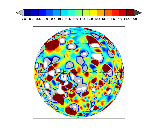 |
| The Triangulate/Trigrid method of gridding to the sphere surface on an orthographic map projection. Something is terribly wrong with this result. |
![]()
Grid to Sphere Surface with GridData and Natural Neighbor Method
There is another method of gridding to the surface of a sphere in IDL. We can use the GridData command in IDL. There are a number of gridding algorithms that can be used in the gridding process. Let's start by using the Natural Neighbor method of gridding. Here is the code we are using.
   Triangulate, lons, lats, triangles
   gridded = GridData(lons, lats, data, /Sphere, Method='NaturalNeighbor', $
       /Degrees, Dimension=[720, 360], Triangles=triangles)
   x = cgScaleVector(Findgen(720), 0, 360)
   y = cgScaleVector(Findgen(360), -90, 90)
   cgDisplay, Title='Spherical Gridding with Natural Neighbor', WID=2, 900, 750
   cgMap_Set, /ORTHOGRAPHIC, 0, 180, Position=[0.1, 0.1, 0.9, 0.8], /ISOTROPIC
   cgContour, gridded, x, y, /OVERPLOT, /CELL_FILL, C_COLORS=c_colors, Levels=levels
   cgMap_Grid, LatDel=20, LonDel=40, /Label
   cgColorbar, NColors=nlevels, OOB_Low=0b, Range=[7.5,15.0], Divisions=nlevels, $
       /Discrete, Format='(F0.1)', Bottom=1, OOB_High=Byte(nlevels+1), $
       Position=[0.1, 0.88, 0.9, 0.93]
You see the results in the figure below. The gridded output from this method has a range of 0.0000 to 14.1783, which compares favorably to the original data range, and you can clearly see that the output matches what we were expecting when we displayed the original data in the cylindrical projection in the first figure.
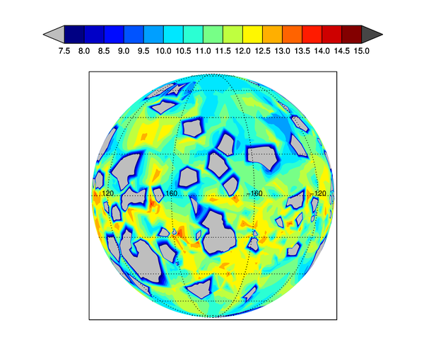 |
| The Natural Neighbor method of gridding to the sphere surface with GridData on an orthographic map projection. |
![]()
Grid to Sphere Surface with GridData and Inverse Distance Method
If you wish, you can use other gridding algorithms with the GridData command. In this example, we use the Inverse Distance method. You can see from the figure below that this gives the appearance of better resolution, because of the interpolated values. Here is the code.
   Triangulate, lons, lats, triangles
   gridded = GridData(lons, lats, data, /Sphere, Method='inversedistance', $
       /Degrees, Dimension=[720, 360], Triangles=triangles)
   x = cgScaleVector(Findgen(720), 0, 360)
   y = cgScaleVector(Findgen(360), -90, 90)
   cgMap_Set, /ORTHOGRAPHIC, 0, 180, Position=[0.1, 0.1, 0.9, 0.8], /ISOTROPIC
   cgContour, gridded, x, y, /OVERPLOT, /CELL_FILL, C_COLORS=c_colors, Levels=levels
   cgMap_Grid, LatDel=20, LonDel=40, /Label
   cgColorbar, NColors=nlevels, OOB_Low=0b, Range=[7.5,15.0], Divisions=nlevels, $
       /Discrete, Format='(F0.1)', Bottom=1, OOB_High=Byte(nlevels+1), $
       Position=[0.1, 0.88, 0.9, 0.93]
You see the result in the figure below.
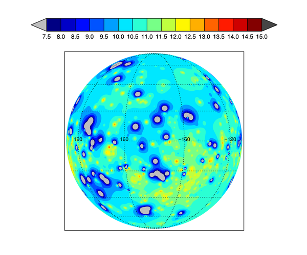 |
| The Inverse Distance method of gridding to the sphere surface with GridData on an orthographic map projection. |
I think the bottom line here is that if you want to grid to the surface of a sphere, you would be well advised to use GridData for the purpose and to avoid the Triangulate/Trigrid method.
![]()
Version of IDL used to prepare this article: IDL 8.2.2.
![]()
![]()


