
Speeding Up Filled Contour Plots


QUESTION: Creating a filled contour plot with my data is taking forever! Is there a way to speed this up?
Here is an IDL save file with the data itself. After you restore it, you will have the variables data, x, and y. It is these variables I am trying to contour. My code looks like this.
   Restore, File='fastfill.sav'
   levels = [0,2,5,10,15,20,25,30,35,40,50,60,75,100,150,200,300]
   cgLoadCT, 16, NColors=16, Bottom=1
   TVLCT, 255, 255, 255, 0
   names = [StrTrim(levels,2), ' ']
   names[16] = '300+'
   cgContour, data, x, y, Levels=levels, C_Color=Indgen(17), $
       Position=[0.1, 0.1, 0.9, 0.8], /Cell_Fill
   cgColorbar, /Discrete, NColors=17, Ticknames=names
This code results in nice output (see below), but it is taking somewhere in the neighborhood of 80-100 seconds to render! I'm already drowning in coffee and I can't drink another one. Isn't there something I can do to speed this up?
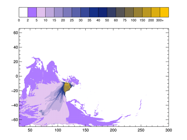 |
| A filled contour plot that takes 80-100 seconds to render. |
![]()
ANSWER: This is a pretty big data set. The data variable is a 4051 x 2032 float array. I expect some slowness with that much data. But, there doesn't seem to be any particular reason here to use the always slower Cell_Fill keyword (which must be used when putting contours on maps to get the contour colors correct). Since we don't have a map here, my first inclination is simply to use the Fill keyword instead of the Cell_Fill keyword with the contour command.
   cgContour, data, x, y, Levels=levels, C_Color=Indgen(17), $
       Position=[0.1, 0.1, 0.9, 0.8], /Fill
   cgColorbar, /Discrete, NColors=17, Ticknames=names
This, in fact, does speed things up. This command now renders in 4-5 seconds, but as you can see from the figure below, doesn't look anything like the previous plot!
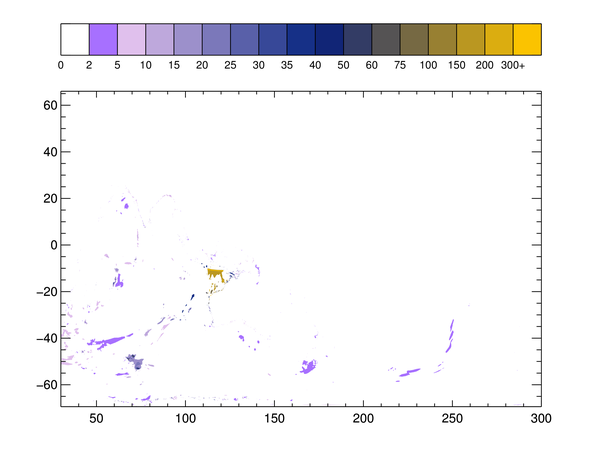 |
| A filled contour plot that is reasonably fast to render, but wrong! |
I really don't have any explanation for why the filled contours are different in this plot. But, in fooling around with this problem to see if I could understand it, I noticed that I was getting some floating point errors as I was working with the data. For example, I typed this.
   IDL> minmax, data
   MinMax:      0.000000      474.000
   % Program caused arithmetic error: Floating illegal operand
That's a strange error. So I thought I would just make sure that the minimum value of this data was actually zero, and then I tried the command again with the Fill keyword. Lo and behold, that fixed whatever had previously been "wrong!"
[I learned later, from Josh, a technical support engineer at Excelis, that the "fix" I discovered was really doing nothing more than turning NaNs in the original data set into zeros. Doh! I even had a note on page 161 of my IDL graphics book explaining this. Maybe I should read the darn thing! The bottom line is that the Cell_Fill keyword algorithm can handle NaNs reasonably well, but the Fill keyword algorithm can't. I'll remember that next time.]
   data = data > 0.0
   cgContour, data, x, y, Levels=levels, C_Color=Indgen(17), $
       Position=[0.1, 0.1, 0.9, 0.8], /Fill
   cgColorbar, /Discrete, NColors=17, Ticknames=names
Now, I see the same result I saw before and I am rendering the contour plot about 20 times faster than I was with the Cell_Fill keyword.
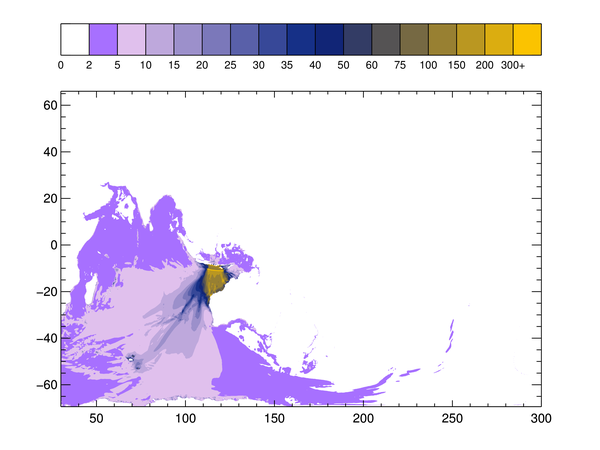 |
| A filled contour plot with whatever was wrong with the data fixed! It rendered in about 5 seconds. |
Four to five seconds is still pretty slow to render a contour plot. Unless, of course, you are talking about the new function graphics Contour function. It would be extremely fast for that graphics routine! Nevertheless, I would like to speed this up some more, if possible.
A filled contour plot is very much like a partitioned image, so I thought I would try to display this as an image, rather than as a filled contour plot. I used Value_Locate to partition the image, and I displayed it like this.
   scaledData = Byte(Value_Locate(levels, data))
   cgImage, scaledData, Position=[0.1, 0.1, 0.9, 0.8], $
      XRange=[Min(x), Max(x)],$
      YRange=[Min(y), Max(y)], /Axes
    cgColorbar, /Discrete, NColors=17, Ticknames=names
This plot rendered in less than 0.2 seconds and, as you can see in the figure below, looks identical to the filled contour plots. Clearly, this is the fastest way to render this data.
 |
| A partitioned image as a filled contour plot renders in 0.2 seconds. |
![]()
Filled Contours on Map Projections
It turns out that the person requesting this information wanted to display this filled contour on a map. (The x and y variables are actually longitude and latitude values.) This is easily done with Coyote Graphics map projection routines. Here is the code I used to put this on a map projection.
   xrange = [x[0], x[N_Elements(x)-1]]
   yrange = [y[0], y[N_Elements(y)-1]]
   limit = [yrange[0], xrange[0], yrange[1], xrange[1]]
   centerLon = (xrange[1] - xrange[0]) / 2.0 + xrange[0]
   centerLat = (yrange[1] - yrange[0]) / 2.0 + yrange[0]
   scaledData = Byte(Value_Locate(levels, data))
   cgImage, scaledData, Position=[0.1, 0.1, 0.9, 0.8], /Erase
   map = Obj_New('cgMap', 'Equirectangular', Center_Lon=centerlon, LIMIT=limit, /OnImage)
   map->Draw
   cgMap_Continents, /Fill, Color='Charcoal', Map=map
   cgMap_Grid, Color='Charcoal', Map=map, /Label, LatLab=200
   cgColorbar, /Discrete, NColors=17, Ticknames=names
Here is the result of the filled contour plot (as a partitioned image) on a map projection.
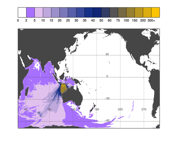 |
| A partitioned image as a filled contour plot in a map projection. |
Chris Torrence has supplied me with code that displays the image on a map using the IDL 8.1 function graphics system. The code looks like this, without the color bar, since a color bar of this type will not be available until IDL 8.2 is released. (I added the map grid to the map, it was not in Chris's original code.)
  TVLCT, rgb, /Get
  scaledData = Byte(Value_Locate(levels, data))
  im = IMAGE(scaledData, x, y, RGB_TABLE=rgb, $
    XRANGE=xrange, YRANGE=yrange, GRID_UNITS='degrees')
  mc = MapContinents(COLOR='dark gray', /FILL)
  mg = MapGrid(COLOR='dark gray')
You see the result below. Notice that half the map seems to be missing. This was the reason for adding the map grid lines. I wanted to confirm that all of the continental outlines to the right of the International Date Line are missing. Note also that the continents are rendered in black rather than the requested dark gray color, and that the grid does not appear to be confined to the image boundaries. I presume these are bugs that will be fixed in IDL 8.2.
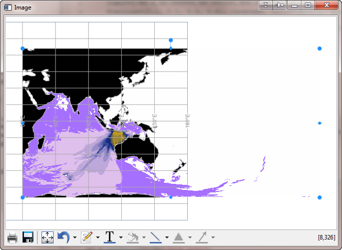 |
| A partitioned image displayed on a map in function graphics. |
Alain Lecacheux helped us out with the IDL 8.x code. It turns out that the default longitude range in MapContinents is -180 to 180 degrees, while our data is in the range 0 to 360. This can be solved by overplotting a suitable map on top of the image. The code will look like this.
  tvlct, rgb, /Get
  scaledData = Byte(Value_Locate(levels, data))
  im = IMAGE(scaledData, x, y, RGB_TABLE=rgb, XRANGE=xrange, $
     YRANGE=yrange, GRID_UNITS='degrees', POSITION=[0.1,0.1,0.9,0.9], $
     ASPECT_RATIO=0)
  mp = map('EQUIRECTANGULAR', LIMIT=limit, LABEL_POSITION=0, $
         POSITION=[0.1,0.1,0.9,0.9], /CURRENT, ASPECT_RATIO=0)
  mc = MapContinents(FILL_COLOR='dark gray', LIMIT=limit)
  grid = mp.mapgrid
  grid.color='dark gray'
  grid.label_color='black'
  grid.linestyle = 2
  grid.transparency = 15
Alain notes the use of the Fill_Color, instead of the Color keyword, to get the continents the right color. He points out that there are no bugs here, but tricky useage of partly undocumented keywords. The result is shown below.
For my part, I note that the Aspect_Ratio keyword documentation for the Image() function is wrong (well, exactly wrong, so if you can think backwards that will help). And, the Aspect_Ratio keyword is not documented at all for the Map() function, but without it you will get a image and map that will cause you to tear your hair out for days!
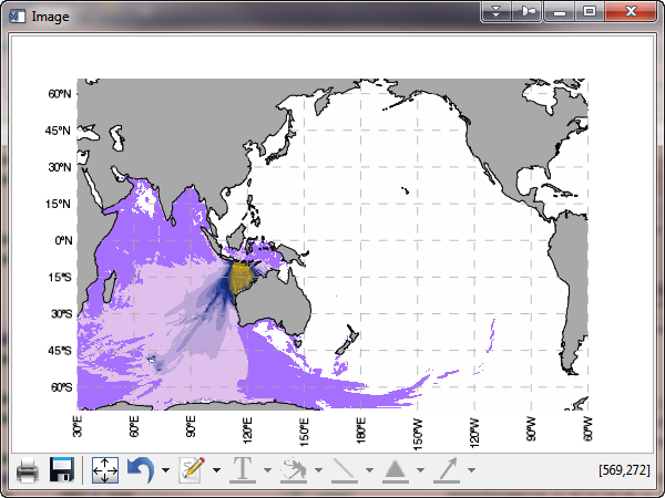 |
| A partitioned image displayed correctly on a map in function graphics. |
![]()
Version of IDL used to prepare this article: IDL 8.1.
![]()
![]()


