Active Contouring (Snakes) in IDL

QUESTION: Is it possible to create an active contour or a snake in IDL?

ANSWER: Yes, it is possible. I've been interested in this topic lately and have written an active contouring application that can be used with a number of my medical image processing programs. In order to introduce IDL users to this topic, I have put together a demonstration program that can be run on the IDL Virtual Machine for those of you who do not yet have a copy of IDL 6.0. (The Virtual Machine can be downloaded free from Research System's web page if you don't already have a copy.) The demonstration program is not fully-functional, but does contain enough functionality for you to see if active contouring will work for you. You can use your own images in the demonstration program.

Updates...

The Active Contouring software has now been updated to work with Coyote Graphics routines. The programming interface and the algorithm itself have been improved, as has the on-line documentation.

Also, several people have asked for a non-interactive version of the program that they can use in batch processing of many files. This is now available as the function cgSnake. This program requires the object program GVF_Snake, which can be purchased at the Coyote Store.

I have done a fair amount of research on active contouring, and I think one of the best active contouring methods was developed by Chenyang Xu and Jerry Prince. They discuss their method and their results on their Active Contours and Gradient Vector Flow web page. The heart of their active contouring method is the Gradient Vector Flow, which provides the external force necessary to push the active contour toward the image edges. I have implemented the method outlined by Xu and Prince in their paper in the IEEE Transactions on Image Processing, Vol. 7, No. 3, entitled Snakes, Shapes, and Gradient Vector Flow, in my ActiveContour IDL program.

The ActiveContour program comes in a zip file. Create a new directory for these files, perhaps named activecontour. Extract all the files in the zip file into this new directory and add the directory to your IDL Path. You will find these five directories. Note, you will also need to download and install the Coyote Library to run the ActiveContour programs.

help	A directory containing the program help file.
images	A directory containing sample images files.
parameters	A directory containing parameter definition files.
roi	A directory containing final contour examples.
source	A directory containing the activecontour.sav file.

Drag the activecontour.sav onto the IDL Virtual Machine to run the program. (Or, alternatively, just type "activecontour" at your IDL prompt.)

Running the Active Contour Program

Once installed, you run the program like this:

   IDL> ActiveContour

Or, if you have the IDL Virtual Machine, just drag the ActiveContour icon onto the Virtual Machine icon. Off you go.

You will be asked to select an example image file from the images directory. If you like, you can browse to any directory that holds image files. The program can work with 2D images stored in BMP, DICOM, JPEG, PGM, PNG, and TIFF format files. The image selection tool looks like this.

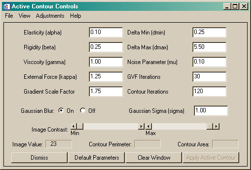
Once you have selected an image, it will be displayed in a separate window and the ActiveContour control panel will appear, as shown below. From the control panel, you can control the internal and external force parameters, other active contouring parameters, as well as manipulate the image before active contouring takes place. For example, the Image Contrast sliders will allow you to manipulate image contrast, and you can find smoothing functions listed under the Adjustments menu button.

The Apply Active Contour button does not become sensitive until an initial contour has been drawn in the image display window.

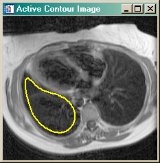
Once you have manipulated the image (it may not need any or much manipulation), you can move your cursor into the image display window and select the starting coordinates for the active contouring algorithm. You will need at least three non-linear points to create an initial contour. Use your left or middle mouse button to select the points. You can close the contour curve by either clicking with the right mouse button, or by double clicking either the left or middle mouse button inside the image.

When you close the initial contour curve, you will see the curve smooth itself slightly. This is normal and is required for subsequent active contour processing.

If you wish to choose another curve, just continue to click in the image window with your left or middle mouse button. The first curve will be discarded and the algorithm will use the curve you are drawing now as its initial active contour position. You can experiment with the ActiveContour parameters and the initial contour position to see how far away from the final contour you will need to position the initial contour. In general, you have be close but not so close that you have to be meticulous in selecting the initial contour.

Once you hit the Apply Active Contour button, you will see the active contour begin to snake around to its final position. You see an intermediate stage in the figure below.

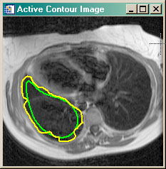
The intermediate active contour is shown in yellow, while the initial contour is shown in green. This initial contour was well chosen, so the final contour converges quickly in about 25 iterations.

Active Contour Parameters

Active contours are like the little girl in the story who "when she was good, was very, very good, but when she was bad, was horrid." That is to say, it is sometimes a challenge to get good active contour parameters in order to obtain acceptable results. You get better with experience. The only good way to understand the parameters is to experiment with them and see how they affect the final contour. The ActiveContour program is designed to make this process as interactive and as easy as possible.

Here are the parameters you can set interactively from the control panel as shown in the figure above.

Elasticity	The elasticity is known as the property alpha in the Xu and Prince paper cited above. Its value can be set with the Alpha keyword when calling the program from the IDL command line. The elasticity force acts to keep the curve from stretching. Larger values make the contour harder to stretch along its length.
Rigidity	The rigidity is known as the property beta in the Xu and Prince paper. Its value can be set with the Beta keyword when calling the program from the IDL command line. The rigidity force acts to keep the curve from bending too much, as, for example, when turning a corner. Larger values make the curve "stiffer" or harder to bend.
Viscosity	The viscosity is known as the property gamma in the Xu and Prince paper. Its value can be set with the Gamma keyword when calling the program from the IDL command line. The viscosity controls how quickly and how far the curve can be deformed between iterations. Larger values make the curve harder and slower to deform. If you see the curve "jumping around", increase the viscosity
External Force	The external force is known as kappa in the Xu and Prince paper. Larger values cause a stronger force toward the image edges. The value can be set with the Kappa keyword.
Gradient Scale Factor	The external force field "pushes" the curve toward edges in images. Edges are where image values change quickly from dark to light and visa versa. The force is calculated in terms of a gradient or first derivative operator. This factor simply multiplies the gradient force fields by this factor before they are used to calculate the Gradient Vector Flow (GVF). The value can be set with the GradientScale keyword.
Delta Min / Delta Max	As the curve is deformed, points are either added to the curve or subtracted from it (so the curve can expand and contract). These factors determine the minimum and maximum pixel distance between adjacent points in the curve. If two adjacent points are further apart than the maximum, a point is added between them. If two adjacent points are closer together than the minimum, then one of the points is eliminated. You might have to play with these parameters depending upon the size of your original image and initial contour. These parameters are knows as dmin and dmax in the Xu and Prince paper, and can be set with the DMin and DMax keywords.
GVF Iterations	The Gradient Vector Flow fields are derived from the image by minimizing a pair of decoupled linear partial differential equations that diffuses the gradient vectors (in X and Y) of the image. This minimization must be done only once for each image (assuming the image doesn't change in appearance). The solution is arrived at iteratively. The default number of 30 is usually sufficient to arrive at a minimized solution, although it could be that 10 or 15 iterations will suffice. In any case, the ActiveContour program only performs the calculation when necessary to improve interactivity. Set this value with the GVF_Iterations keyword.
Contour Iterations	This is the number of times the active contour is deformed according to the internal and external force fields and then "processed" by the program to obtain the next starting contour location. The default is 120, but most active contours will settle to a stable configuration in far fewer iterations. You can click the Accept button on the Contour Iteration progress bar to accept the current configuration, even if you haven’t reached the end of the iterations. Set this parameter with the Iterations keyword.
Noise Parameter	The noise parameter is known as the property mu in the Xu and Prince paper. Its value can be set with the Mu keyword. The noise parameter governs the way the GVF field is calculated. Basically, this parameter should be set to higher values in noisy images and to lower values in normal images.
Gaussian Blur	Often the image gradients are more distinct, and provide a better GVF external force field, if a Gaussian smoothing function is applied to the image prior to calculating the image gradients. The default is to include this image smoothing.
Gaussian Sigma	The sigma or overall shape of the Gaussian smoothing is set with this factor, called sigma in the Xu and Prince paper. A larger value of sigma results in smoother image than with a small value of sigma. The default is 1.0 and the parameter can be set with the Sigma keyword.
Image Contrast	The image contrast sliders can be manipulated to control the visual contrast in the image. Quite often good separation of features can be obtained, or at least improved, by manipulating image contrast prior to applying the active contour algorithm. Moving the sliders will remove any preliminary active contour currently on the image, so perform image contrast enhancement before drawing the initial active contour. Note that these controls are only available if the ActiveContour program created its own image display window (as it will in the demo version).

Active Contour Menus

In addition to the controls on the face of the control panel, you have other selections from the menu items on the control panel.

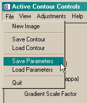
File Menu

The File menu is where you will find the ability to open new image files and to save and restore previously used parameters and active contours. A brief description of each menu item shown in the table below.

New Image	This button allows you to select and open a new image file for display in the image display window. BMP, DICOM, JPEG, PICT, PGM, PNG, and TIFF files can be opened. Note that only 2D images are allowed.
Save / Load Contour	These buttons allow you to save and restore the final contour values. The area and perimeter of the final active contour are stored as well as the contour points themselves.
Save / Load Parameters	It is an effort occasionally to find the right parameters to perform the active contouring adequately. Once you have them, you often want to save them so you can use them again on similar images. These menu buttons allow you to do so.
Quit	This button quits the ActiveContour program and has exactly the same effect as the Dismiss button on the face of the control panel above.

View Menu

The View menu allows you to view some of the intermediate results of the program as an aid to understanding active contouring.

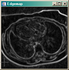
Edgemap	At the heart of the GVF active contouring method is an edgemap. This is the gradient of the image scaled into the range of 0 to 1. What you should see in the edgemap image are the edges of the image. The edgemap is used to calculate the external forces on the contour in the GVF algorithm The active contour is 'pushed" or "pulled" toward the image edges.
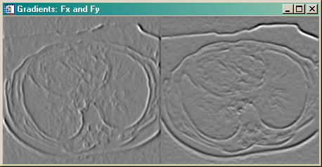
Gradient Fields	The forces used in GVF active contouring are produced by gradient fields. To be useful, these fields need to be calculated in the X and Y directions. This menu item will show you the Fx and Fy gradient images.
Vector Field	This button will allow you to view the vector force field (i.e., a plot of Fx vs. Fy) that is pushing the contour toward the image edges. Note that the vectors are strongest near the image edges and nearly perpendicular to the edges, as well

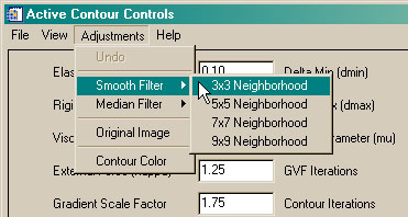
Adjustments Menu

The Adjustments menu allows you to smooth the image in various ways prior to calculating the active contour. This menu item is only available when the ActiveContour program creates its own image display window.

Undo	This button removes either a Smooth or a Median filter operation in the opposite order in which they have been applied to the image. The button is only sensitive when there is a process to undo.
Smooth Filter	This button allows you to apply a Smooth filter of various sizes to the image. Note that once a filter is applied, it can be removed by the Undo button.
Median Filter	This button allows you to apply a Medianfilter of various sizes to the image. Note that once a filter is applied, it can be removed by the Undo button.
Original Image	This button restores the original image in the image display window and discards any filter operations that have previously been applied to the image.
Contour Color	This button will allow you to change the color used to draw the initial and final contours

Help Menu

The Help menu offers two kinds of help documents.

User's Guide	An ActiveContour User's Guide, presented in PDF format.
Program Documentation	Complete program documentation for all the programs in the ActiveContour application. Presented in HTML format.

Full-Featured Active Contour Program

The ActiveContour IDL source code is available to purchase. Note, you will also need to download and install the freely available Coyote Library to run the ActiveContour programs.