Displaying Gridded Land Cover Data

QUESTION: Can you help me? I have some gridded land cover data that has been gridded into a polar stereographic map projection. I have the corresponding latitude and longitude arrays to go with each pixel of the gridded land cover data, but I don't have the foggiest idea what to do with them, or how to display the data in IDL.

Here is what I know. The data was read out of a netCDF file created by a colleague. The data is gridded on a polar stereographic map projection. Here are the details of the map projection that were in the netCDF data file.

   grid_mapping_name = polar_stereographic
   straight_vertical_longitude_from_pole = -115.000
   standard_parallel = 60.0000
   false_easting = -630000.
   false_northing = 4.64850e+006
   latitude_of_projection_origin = 90.0000
   resolution_at_standard_parallel = 45000.0

I read the data out of the netCDF file and stored the data into text files that I am sending you in a zip file. The data files were defined in the netCDF file like this.

   lat = FltArr(91,67)
   lon = FltArr(91,67)
   gc  = FltArr(91,67)

Other useful information in the file are the values of the ground cover. The file contains this information.

   -1 - ground
    0 - ocean
    1 - seaice 
    2 - ice free lake
    3 - lake ice

ANSWER: OK, I'll try to help, but I can tell you right off the bat, something is odd here. Ground cover data that has integer values should not be in a floating point array. And inspection of the gc.txt file (located, if you want to follow along in the zip file) shows plenty of -1 values, but no zeros and no integers. My guess is the netCDF file created by your colleague was not created correctly. This is a common enough occurance, but you might want to contact your colleague to see what is going on. Since the data is a two-dimensional array it is convenient to think of it as an "image," and I will use this term interchangably with "data" in the discussion that follows.

Another problem is that the map projection information is incomplete. For example, while we know this is a polar stereographic map projection, we are not told what datum was used with the map projection. I'm going to assume this is satellite data and that a WGS84 datum was used. But, if some other datum was used when the data was gridded, we will be off when we annotate the image with latitude and longitude values (since the choice of datum determines where the latitude and longitude values are actually located).

I have witten a program to read and display the data, which I will discuss here. The program uses Coyote Graphics map projection routines, which I use to work around numerous problems with IDL's own routines.

Read and Reverse the Data

The first step is to read the data files. I assume the data files have been unzipped and are in the same directory as the file that will read them. The code is relatively simple. The only unusual thing here is that we immediately reverse the data in the Y direction when we read the file. This is because all mapping software in the world (aside from IDL) puts the origin, or (0,0) point of the image, in the upper left corner of the image, whereas IDL puts the origin in the lower left corner of the image. By reversing the image in the Y direction, we will put the origin in the generally accepted correct upper-left position. I would say this reversal has to be done about 95-98 percent of the time when you are reading data sets that were not created in IDL but have been gridded using some kind of a map projection.

   latFile = cgSourceDir() + 'lat.txt'
   lonFile = cgSourceDir() + 'lon.txt'
   gcFile  = cgSourceDir() + 'gc.txt'
   
   ; Read the data. Data going onto map projections must
   ; almost always be reversed in the Y direction.
   OpenR, lun, latFile, /GET_LUN
   header= ""
   lats = FltArr(91,67)
   ReadF, lun, header, lats
   Free_Lun, lun
   lats = Reverse(lats,2)
   
   OpenR, lun, lonFile, /GET_LUN
   header= ""
   lons = FltArr(91,67)
   ReadF, lun, header, lons
   Free_Lun, lun
   lons = Reverse(lons, 2)
   
   OpenR, lun, gcFile, /GET_LUN
   header= ""
   gc = FltArr(91,67)
   ReadF, lun, header, gc
   Free_Lun, lun
   gc = Reverse(gc,2)

Set Up the Map Projection

The next step is to set up the polar stereographic map projection. The polar stereographic projection in IDL is a strange one. The projection is obviously centered at the pole (I assume the north pole, in this case, although the data in the file doesn't mention this, and I am assuming it from your Canadian e-mail address.) Polar stereo projections have a latitude of true scale. Normally, this is set with the TRUE_SCALE_LATITUDE keyword, although up through IDL 8, this latitude of true scale was set with the CENTER_LATITUDE keyword, and the TRUE_SCALE_LATITUDE keyword was flagged as being not supported for polar stereo map projections. The CENTER_LATITUDE keyword will still set the latitude of true-scale in IDL 8, but it is also now possible to do this correctly with the TRUE_SCALE_LATITUDE keyword. Since I don't know which version of IDL you are using, I'll use the incorrect form of the command, although it will work properly in all versions of IDL.

Note that I am using Map_Proj_Init, rather than Map_Set, to set up the map projection space. Map_Proj_Init, while not state-of-the-art with respect to map projections, uses the professional quality (well, 20 years ago) GCTP projection code from the USGS. The Map_Set command is not of sufficient quality to be used for most professional mapping problems. The Map_Proj_Init command returns a map structure variable that I will use in subsequent commands.

We will have to guess a little bit about what the map projection information provided you actually means. It is clear that the "straight_vertical_longitude_from_pole" is the center latitude of the map projection. Normally, the latitude of true-scale is 70 degress with polar stereo map projections, so I am going to assume that "standard_parallel = 60.0000" is really the latitude of true-scale. The false-easting and false-northing information is safe to ignore. We are going to find the XY Cartesian coordinates of the image in another way. We set the map projection like this, assuming a WGS84 datum (ELLIPSOID=8). The ONIMAGE keyword is set so that the cgMap object will get its position from the position the image is in after it is displayed.

   map = Obj_New('cgMap', "Polar Stereographic", ELLIPSOID=8, $
      CENTER_LONGITUDE=-115, CENTER_LATITUDE=60.0, /ONIMAGE)

Find the "Box" that Surrounds the Image

Some software will use the latitude and longitude arrays provided with the data to position the data in the map projection space. We will do that, too, but probably in a different way from most mapping software. Really, since this is gridded data, I am interested in knowing only the latitude and longitude locations of the four corner pixels, since I can use this to calculate a "box" that my image will fit in. Here is how I use the corners and convert the latitude/longitude values to XY Cartesian coordinates with Map_Proj_Forward. Notice the MAP_STRUCTURE keyword is an input keyword that accepts the map structure variable obtained from the cgMap object. I will use this map structure again later when I want to annotate the data.

   lonCorners = [lons[0,0], lons[90,0], lons[90,66], lons[0,66]]
   latCorners = [lats[0,0], lats[90,0], lats[90,66], lats[0,66]]
   xy = Map_Proj_Forward(lonCorners, latCorners, MAP_STRUCTURE=map->GetMapStruct())

We have one problem. The latitude and longitude locations are undoubtably given at the data pixel centers. I want to have a box that surrounds the pixels. If I use the pixel centers to create my box, I am exactly one pixel too short in both the X and Y directions. Thus, to create the proper box, I have to subtract half a pixel's distance from one end of the box, and add half a pixel's distance to the other end of the box. First, I have to know the distance of each pixel in the X and Y directions. I'll call this the xscale and yscale, and I can obtain the values from the corner pixels and the dimensions of the data.

   s = Size(gc, /DIMENSIONS)
   xscale = Abs((xy[0,1] - xy[0,0]) / (s[0]-1))
   yscale = Abs((xy[1,3] - xy[1,0]) / (s[1]-1))

Finally, I'll add the appropriate half pixel to each end of my box. The point (x0,y0) will be at the origin (upper left) and the point (x1,y1) will be opposite it (lower right) of the "box" that will contain the data.

   x0 = xy[0,0] - (xscale/2.0)
   x1 = xy[0,1] + (xscale/2.0)
   y0 = xy[1,0] - (yscale/2.0)
   y1 = xy[1,3] + (yscale/2.0)

Display the Image Data

The next step is to display the data. Since I am not quite sure why this land cover data is not integer data, as it is described in the file, I will round the values found in the file, and then add 1 to each value, to obtain values that go from 0 to 4. In other words, I will have five distinct values in the file after rounding. (I am not sure this is the correct way to proceed, but the information provided me is contradictory and impossible to interpret.)

Before I display the data as an image, I'll load five colors into the color table to use for the five land cover values I expect to display. The code looks like this. Notice I define a position for the data in the display window in a way that will leave room for a color bar later on.

   TVLCT, cgColor(['sienna', 'dodger blue', 'honeydew', 'ygb5', 'pbg3'], /TRIPLE)
   p = [0.05, 0.05, 0.95, 0.8]
   cgImage, Round(gc)+1, /KEEP_ASPECT, /ERASE, POSITION=p

The next step is the one most often overlooked by IDL programmers. We want to set up a coordinate system for the image that exactly overlaps the image in space. The reason for doing this is so that we can annotate the image will other information, such as continental outlines, map grid values, etc. Doing the annotation is an excellent check to see if we have set up the map projection properly. If map annotations don't line up with features in the data, then something is amiss.

We have to tell the cgMap object what its range will be, since it will be responsible for setting up the data coordinate system in projected meter space. It will get its position from the last position set with cgImage displayed the image. We can create the data coordinate space by setting the DRAW keyword, which will call the Draw method on the object after its parameters are set.

   map -> SetProperty, XRANGE=[x0,x1], YRANGE=[y0,y1], /DRAW

Annotate the Image

Next, we annotate the image. What you do here is up to you. I want to draw some continental and USA outlines and add map grids. My code looks like this.

   cgMap_Continents, MAP_STRUCTURE=map, COLOR='gray'
   cgMap_Continents, MAP_STRUCTURE=map, COLOR='gray', /USA
   cgMap_Grid, MAP_STRUCTURE=map, COLOR='white', /LABEL, $
        LATS=Indgen(9)*10, LONS=Indgen(10)*10-130

Add a Color Bar

The final step is to add a discrete color bar.

   cgDCBar, NCOLORS=5, BOTTOM=0, $
        LABELS=['Land', 'Ocean', 'Sea Ice', 'Lake', 'Lake Ice']

The final result is shown in the figure below. It looks like the choices we made with the data and the map projection were good ones, as the data is well-aligned. We are looking at the Great Lakes in the lower center of the image, and the famous Hudson Bay, now covered in ice, in the center left of the image. Shore ice is also easily distinguished.

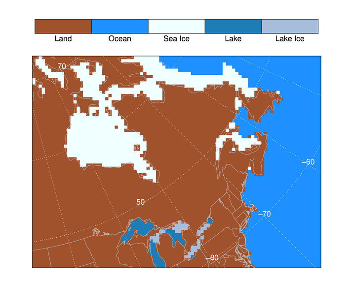The land cover data displayed in a polar stereographic map projection.

 

Version of IDL used to prepare this article: IDL 7.0.1.