
Map Function Knows No Bounds
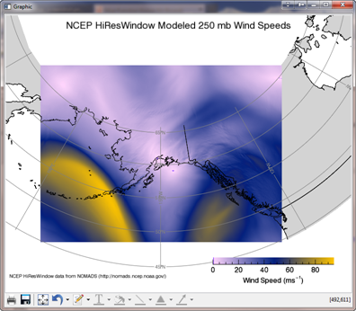
QUESTION: Mark Piper shows how to display some wind speed data as an image on a map in an article on his IDL blog. Here is a representation of that data.
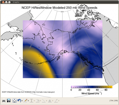 |
| Wind speed data displayed as an image on a map projection. |
Normally, I would want to display this kind of data in a rectangular region of the display window, with the map projection coincident with the the image data. I've tried to modify Mark's code to get what I want, but so far I have been unsuccessful. Mark sets up his map projection like this.
   m = map('Polar Stereographic', $
      /current, $
      semimajor_axis=r_u250.radius, $
      semiminor_axis=r_u250.radius, $
      true_scale_latitude=r_u250.ladindegrees, $
      center_longitude=r_u250.orientationofthegridindegrees, $
      position=[0.1,0.1, 0.8, 0.9], $
      color='gray')
Then, a bit later in the code he sets the map limits and scale like this.
   m.limit = [40, 150, 80, 270]
   m.scale, 2.0, 2.0, 1.0
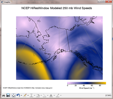
I reasoned from the documentation that I could use the XRANGE and YRANGE keywords instead of the LIMIT and SCALE keywords to get what I wanted from the values in Mark's code. I commented out the two lines above and substituted these lines.
   xrange = [xy0[0],xy0[0]+xsize]
   yrange = [xy0[1],xy0[1]+ysize]
   m.xrange = xrange
   m.yrange = yrange
Later, he displays the image on the map projection like this.
   i = image(s250, $
      overplot=m, $
      rgb_table=16, $
      grid_units='meters', $
      image_dimensions=[xsize,ysize], $
      image_location=xy0)
But, when I ran the code with my modifications, the result is not what I expected. You see it in the figure below.
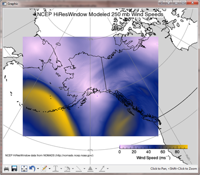 |
| Same display as above with range keywords. |
Am I doing something wrong?
![]()
ANSWER: No, you are not doing anything wrong. If you were doing a similar map projection display in Coyote Graphics, you would do something like this.
    cgLoadct, 16, RGB_Table=pal
    cgImage, s250, /scale, /interp, position=[0.1, 0.1, 0.9, 0.8], $
       palette=pal, /window
    m = cgMap('Polar Stereographic', $
       semimajor_axis=r_u250.radius, $
       semiminor_axis=r_u250.radius, $
       true_scale_latitude=r_u250.ladindegrees, $
       center_longitude=r_u250.orientationofthegridindegrees, $
       xrange=xrange, yrange=yrange,  onimage=1, $
       title='NCEP HiResWindow Modeled 250 mb Wind Speeds')
     grid = cgMapGrid(m, color='gray', thick=1, linestyle=0, $
         label=1, lonlab=62.5, latlab=210)
     continents = cgMapContinents(m, color='black', thick=1, $
          /hires, /countries)
     m.continents = continents
     m.grid = grid
     m.addcmd
You see the result in the figure below.
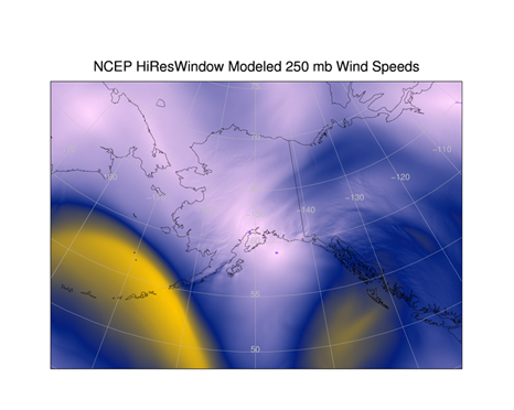 |
| The Coyote Graphics comparable map projection plot. |
But, this kind of map display is not possible in IDL 8.0 or IDL 8.1 because there is a bug in the XRANGE and YRANGE keywords that prevents the map projection from being clipped to that rectangle, as in the figure above.
You could try using the calculated ranges to set the LIMIT keyword to display a smaller subset of the map projection. But this causes other problems. For example, you could set the LIMIT keyword, which requires latitude and longitude values, like this. Note the way you have to rearrage the range that comes back from the MapInverse method to conform to the expected sequence of values in the LIMIT keyword.
   xyrange = [xrange[0], yrange[0], xrange[1], yrange[1]]
   llrange = m.mapinverse(xyrange)
   newLimit = [llrange[1], llrange[0], llrange[3], llrange[2]]
   m.limit = newlimit
Running the code with these modifications results in the figure below. You see several problems, but the most severe is that the continental outlines no longer seem to draw correctly.
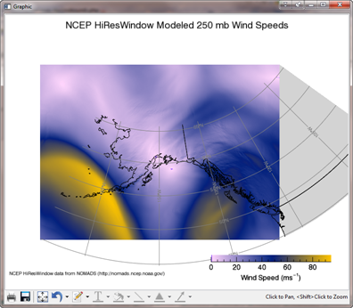 |
| Using the calculated ranges to set the LIMIT keyword, results in other problems. |
You might have better luck if you use the middle of the ranges as the LIMIT values, like this.
   x = [xrange[0], (xrange[1]-xrange[0])/2, (xrange[1]-xrange[0])/2, xrange[1]]
   y = [(yrange[1]-yrange[0])/2, yrange[1], (yrange[1]-yrange[0])/2, yrange[0]]
   llrange = m.mapinverse(x, y)
   newLimit = [Min(llrange[1,*]), Min(llrange[0,*]), Max(llrange[1,*]), Max(llrange[0,*])]
   m.limit = newlimit
Well, as you can see below, maybe not.
 |
| Using the center of the ranges for the LIMIT. |
I guess we are just going to have to wait for IDL 8.2 and hope this problem has been fixed.
The Coyote Graphics map routines I have used here are amoung the dozen or so map projection routines available for the Coyote Graphics Library.
![]()
IDL 8.2 Update
The XRANGE and YRANGE keywords appear to have been fixed in IDL 8.2. Using Mark's orginal program, I simply substituted his limit and scale values:
    m.limit = [40, 150, 80, 270]
    m.scale = 2.0, 2.0, 1.0
With range values that Mark calculated (just below the two commands above), but didn't put together into ranges:
   m.xrange = [xy0[0], xy0[0]+xsize]
   m.yrange = [xy0[1], xy0[1]+ysize]
The result is show in the figure below.
 |
| The XRANGE and YRANGE keywords have been fixed in IDL 8.2. |
![]()
Version of IDL used to prepare this article: IDL 8.1 and 8.2.
![]()
![]()
Updated: 11 Sept 2012


