Colorbar Design Makes Image Comparison Difficult

QUESTION: Maybe it is just me, but I think the design of the IDL 8.1 Colorbar() function makes it extremely difficult, if not impossible, to use in most of the programs where I need a color bar. I am usually doing some kind of image comparison. Can you explain to me why it is a good idea to attach a color bar to a particular plot or image?

ANSWER: Uh, no, I really can't. And I am not sure what to say about the color bar design, except that it seems to have been designed by someone who doesn't actually use color bars in scientific programs. It strikes me as the kind of thing that was designed by a computer scientist, rather than, say, a physical scientist.

In fact, I would go so far as to say that the color bar design is very likely to produce inaccurate and misleading results in the hands of most casual users. I think it is extremely important to know exactly how the color bar function works, and exactly what you are doing if you choose to use this color bar to compare images with different data ranges. The documentation is not clear (well, it is non-existent!) on these important points.

The basic principle of the color bar design is that a color bar should be "attached" to a particular plot or image. This is done by specifying a "target" for the color bar when it is created.

   file = Filepath(SUBDIR=['examples','data'], 'md1107g8a.jpg')
   img = Read_Image(file)
   imgObj = Image(img, Position=[0.1, 0.1, 0.9, 0.8])
   cb = Colorbar(Target=imgObj, Position=[0.1,0.88, 0.9, 0.92])

You see the result in the figure below. Note that the range of the color bar goes from 0 to 255.

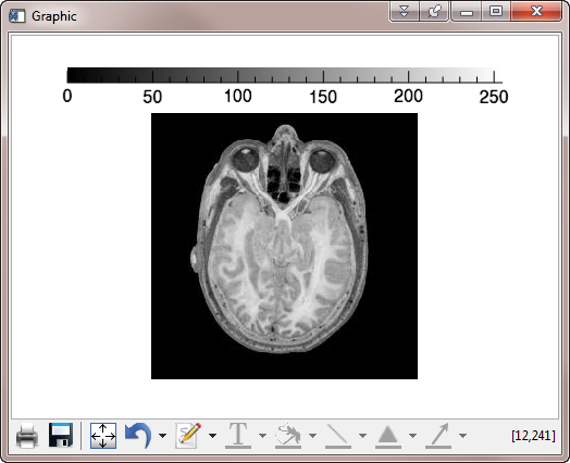In this figure, the color bar range goes from 0 to 255, and the image is assumed to be scaled into the same range.

 

One of the features of the color bar is that it causes the image to be scaled into the color bar range. This may or may not (see below) be a useful feature, but in any case, it is not applied in a consistent manner. It turns out that the color bar range is determined not by the actual values in the image, but by the type of data in the image! Byte data is scaled in a different way than other data types. You can see this by simply converting the byte data used in the figure above to floating point data.

   fimg = Float(img)
   fimgObj = Image(fimg, Position=[0.1, 0.1, 0.9, 0.8])
   fcb = Colorbar(Target=fimgObj, Position=[0.1,0.88, 0.9, 0.92])

As you can see in the figure below, in this case, the data was scaled from 0 to 234, the actual values in the image. Byte data, on the other hand, is always assumed to be scaled into the range 0 to 255.

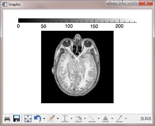The image is scaled and displayed differently, depending upon the type of data in the image. Byte data is always assumed to be scaled into the range of 0 to 255.

 

This point is made more obvious by restricting the data to a narrower data range. Consider this code, in which the data range is forced in the range 80 to 200.

   img = Read_Image(file)
   img = cgScaleVector(img, 80, 200, /Preserve_Type)
   w = Window(Dimensions=[725,475])
   imglt = Image(img, Layout=[2,1,1], /Current)
   lcb = Colorbar(Target=imglt)
   imgrt = Image(Float(img), Layout=[2,1,2], /Current)
   rcb = Colorbar(Target=imgrt)

You see the results below.

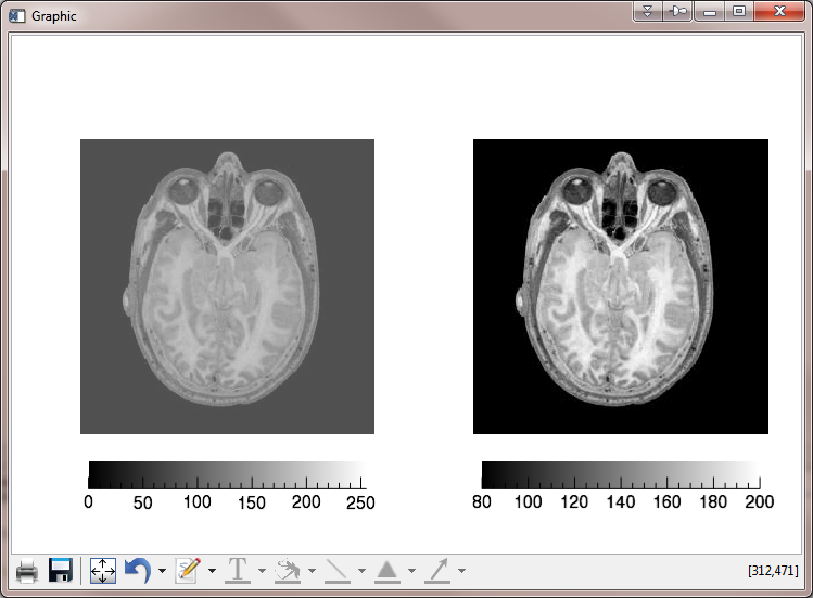The image is scaled and displayed differently, depending upon the type of data in the image, which is made more obvious by restricting the data to a limited data range.

 

Comparing Images

The figure above shows the scaling problem with data of different types, but it foreshadows both the difficulty and solution for displaying two images with different data ranges with a single color bar that reflects the actual values in the two images.

Consider for example, these two floating point data sets.

   data_1 = Congrid(Findgen(10,10), 400, 400)
   data_2 = cgScaleVector(Congrid(Findgen(10,10), 400, 400), 25, 75)

Data set 1 has a data range from 0.0 to 99.0. Data set 2 has a data range from 25.0 to 75.0. Our goal is to compare these two data sets and find the pixels that have a value of, say, 70. We expect the pixels with a value of 70 to have the same "color" in the two data sets.

We first try to display these two data sets in the simplest way, like this.

   w = Window(Dimensions=[775,475])
   i1 = Image(data_1, Layout=[2,1,1], /Current, Axis_Style=2, RGB_Table=33)
   cb1 = Colorbar(Target=i1, /Border_On)
   i2 = Image(data_2, Layout=[2,1,2], /Current, Axis_Style=2, RGB_Table=33)
   cb2 = Colorbar(Target=i2, /Border_On)

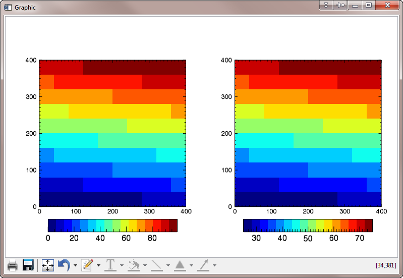
I think it is obvious from the figure below that the the pixels that have a value of 70 in the two images are displayed in different colors. I know by doing a bit of experimenting that the first block of pixels in the row labeled 300 in the left-hand image have values that are 70, and the first two blocks in the top row of the right-hand image have values that are between 70.0 and 71.0. You can see that these blocks are different colors.

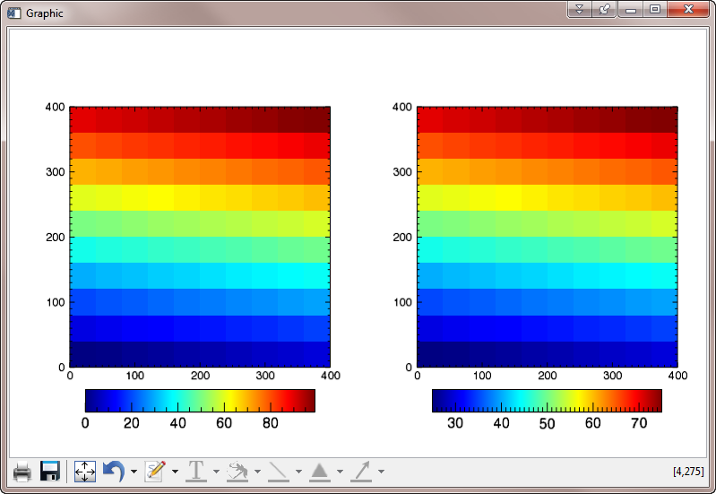Comparing two images with different ranges is impossible using just a simple Colorbar() function attached to the two images. Pixels with a value of 70 are displayed in different colors in the two images.

 

Part of the problem here is that these two data sets are always scaled into 256 colors, according to their respective data ranges. The color bar design makes it impossible to limit the number of colors in the color table. For example, we cannot create a color table that has only 16 colors, unless we fake it by expanding the 16 colors into 256, like this.

   LoadCT, 33, NColors=16, RGB_Table=rgb
   rgb = Congrid(rgb, 256, 3)
   w = Window(Dimensions=[775,475])
   i1 = Image(data_1, Layout=[2,1,1], /Current, Axis_Style=2, RGB_Table=rgb)
   cb1 = Colorbar(Target=i1, /Border_On)
   i2 = Image(data_2, Layout=[2,1,2], /Current, Axis_Style=2, RGB_Table=rgb)
   cb2 = Colorbar(Target=i2, /Border_On)

You see the results in the figure below. You see even more clearly with this restricted-color color table that the data value of 70 is displayed with different colors.

(Please note that with this color bar design, if you are going to restrict the number of colors used, choose a color than can be evenly divided into 256. Otherwise, you will not be able to align your colors and your tick labels (see below) perfectly.)

Creating a color bar with less than 256 colors has to be fudged.

 

To compare images, we want to take advantage of the fact that the color bar displays byte data differently than floating point data and scale the image data ourselves with the BytScl command. It is absolutely imperative that we use the Min and Max keywords as we do this, so that the resulting images are scaled to the same measuring stick. In this case, we want to scale both data sets into the range 0 to 100, and we want to try to display them with 100 colors. (I know I just said not to do this, but bear with me. I have 100 values, I would like to display them in 100 colors!)

  LoadCT, 33, NColors=100, RGB_TABLE=rgb
  rgb = Congrid(rgb, 256, 3)
  data_3 = BytScl(Congrid(Findgen(10,10), 400, 400), TOP=99, MIN=0, MAX=100)
  data_4 = BytScl(cgScaleVector(Congrid(Findgen(10,10), 400, 400), 25, 75), TOP=99, MIN=0, MAX=100)
  w = Window(Dimensions=[775,475])
  i1 = Image(data_3, Layout=[2,1,1], /Current, Axis_Style=2, RGB_Table=rgb)
  cb1 = Colorbar(Target=i1, /Border_On)
  i2 = Image(data_4, Layout=[2,1,2], /Current, Axis_Style=2, RGB_Table=rgb)
  cb2 = Colorbar(Target=i2, /Border_On)

You see the result in the figure below. I would argue that this is data is displayed correctly, and the colors in the color bar are correct, too. But, what has happened to the color bars!?

These images are displayed with the correct colors, and the colors in the color bar are correct, but what happened to the color bars!?

 

To get the color bars to display correctly, we have to scale the data not into 100 colors, but into 256 colors, and we have to use all 256 colors in the color bar. (I realize you may not want to scale your data into 256 colors, but I'm just trying to point out what you have to do to make this work.)

  data_3 = BytScl(Congrid(Findgen(10,10), 400, 400), MIN=0, MAX=100)
  data_4 = BytScl(cgScaleVector(Congrid(Findgen(10,10), 400, 400), 25, 75), MIN=0, MAX=100)
  w = Window(Dimensions=[775,475])
  i1 = Image(data_3, Layout=[2,1,1], /Current, Axis_Style=2, RGB_Table=33)
  cb1 = Colorbar(Target=i1, /Border_On)
  i2 = Image(data_4, Layout=[2,1,2], /Current, Axis_Style=2, RGB_Table=33)
  cb2 = Colorbar(Target=i2, /Border_On)

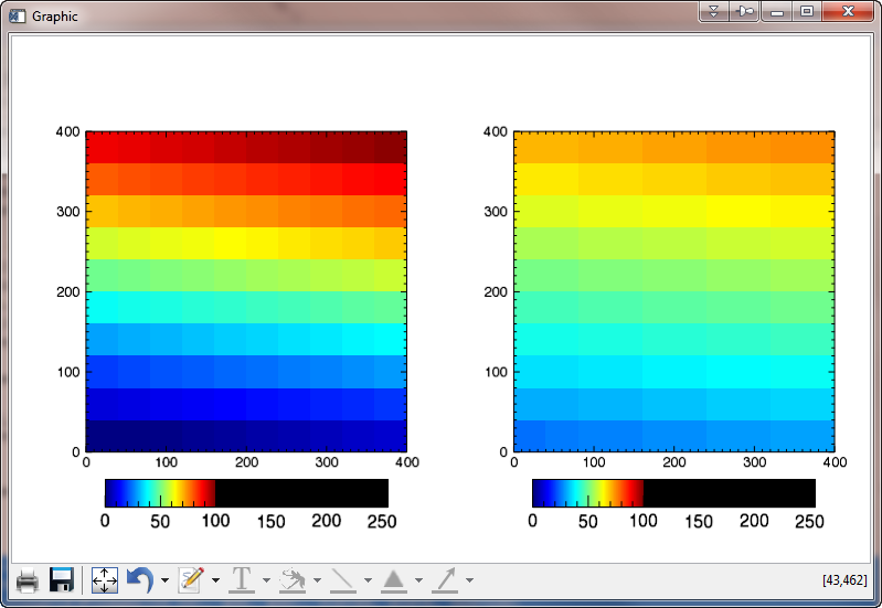
You see the result in the figure below. This figure looks better, except that the color bar labels do not reflect the actual values in the two images.

The image and color bar colors are now correct, but the data values are incorrectly labeled on the color bar.

 

The next step is to label the color bar in such a way that it reflects the actual data values. In our case, we know the data values go from 0 to 100, since this is how we scaled them. We want our color bar to be labeled with these values. There is no way to do this except to physically create the labels that will go onto the color bar in place of the labels the color bar calculates.

In other words, you will have to ignore the actual color bar labels nearly always, and replace the labels with those of your own choosing that will reflect the actual values in your data. The code to do so will look like this. The number of labels you create will be the same as the number of major tick marks you will have to specify for the color bar with the Major keyword. The labels will be specified with the TickName keyword.

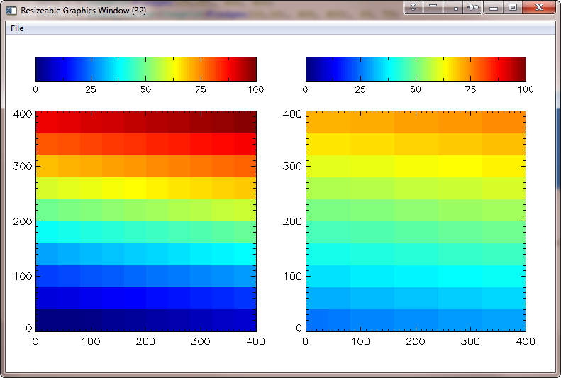
  labels = ['0','25','50','75','100']
  data_3 = BytScl(Congrid(Findgen(10,10), 400, 400), MIN=0, MAX=100)
  data_4 = BytScl(cgScaleVector(Congrid(Findgen(10,10), 400, 400), 25, 75), MIN=0, MAX=100)
  w = Window(Dimensions=[775,475])
  i1 = Image(data_3, Layout=[2,1,1], /Current, Axis_Style=2, RGB_Table=33)
  cb1 = Colorbar(Target=i1, /Border_On, Major=5, Tickname=labels)
  i2 = Image(data_4, Layout=[2,1,2], /Current, Axis_Style=2, RGB_Table=33)
  cb2 = Colorbar(Target=i2, /Border_On, Major=5, Tickname=labels)

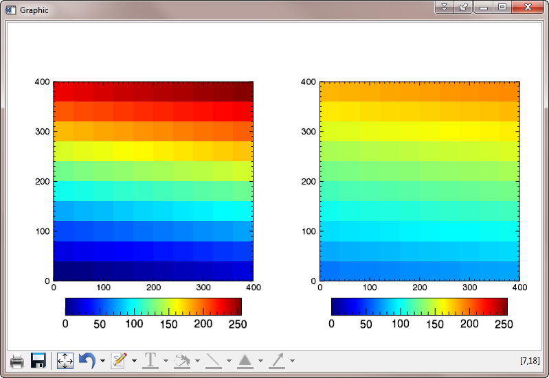
You see the final result in the figure below.

Images and color bars displayed correctly.

 

Rules for Comparing Images

Here are the rules you must follow to compare two images with different data ranges in function graphics.

1. Byte scale your data with the BytScl function, using exactly the same data range with the MIN and MAX keywords. Be sure you scale your data into 256 values.
2. Create image objects of your byte scaled data and make these image objects the targets of the color bars.
3. Ignore the actual values of the color bars, and replace them with string tick labels that you will have to create from the actual data range of the original data and the number of major tick marks you want on the color bar.
4. If you want to use a restricted number of colors in your color bar, choose a number that even divides into 256. Otherwise, you will never be able to match your colors with the values in the image perfectly.

Coyote Graphics Equivalent

Just to compare results, here are the comparable commands in Coyote Graphics, using exactly 100 colors.

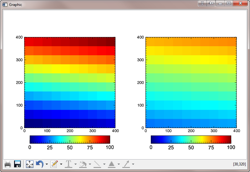
   cgLoadct, 33, NColors=100
   cgWindow, WMULTI=[0,2,1], WXSize=775, WYSize=475
   cgImage, data_1, /Keep, MultiMargin=[2,6,7,5], /Axes, $
	  MinValue=0, MaxValue=100, Top=99, /Add
   cgColorbar, NColors=100, Range=[0,100], Divisions=4, /Fit, /Add
   cgImage, data_2, /Keep, MultiMargin=[2,5,7,6], /Axes, $
	  MinValue=0, MaxValue=100, Top=99, /Add
   cgColorbar, NColors=100,  Range=[0,100], Divisions=4, /Fit, /Add

The result is shown below.

For comparison purposes, here is the same display using Coyote Graphics commands.

 

Version of IDL used to prepare this article: IDL 8.1.