Displaying an Image on a Map Projection

QUESTION: I have some global data I would like to display on a map projection in IDL 8.1, using the function graphics routines, but I can't seem to get it to work. Here is how I've created the image.

   i = Image(data, Grid_Units=2, Map_Projection='Equirectangular', $
       RGB_Table=rgb, Position=[0.05,0.05,0.95, 0.80])

But you can see from the figure below that the map is showing only the northern hemisphere, not the entire globe. Plus, as you can see, my data is upside-down, and I want it to be displayed in 10 distinct colors. What am I doing wrong?

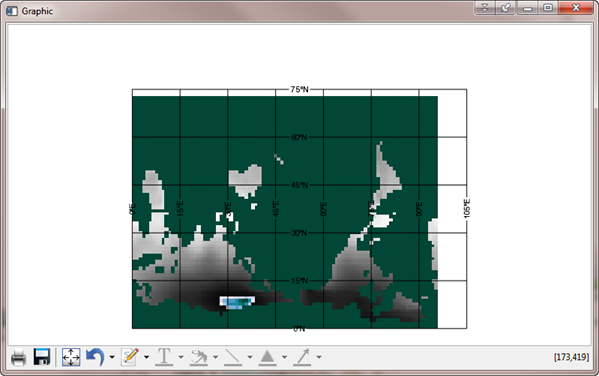The map is showing only the northern hemisphere, and the global data set is upside down.

 

ANSWER: OK, you have several problems here that have to be fixed. First, you are reading the data out of a netCDF file which also has latitude and longitude vectors in the file. You will need the map projection vectors if you plan to display the data correctly on a map projection. Second, data that has been map projected is almost always displayed upside-down in IDL. This is because IDL is the only software package in the world, as far as I know, that puts the origin of the map coordinate system in the lower-left corner of the display. All other software puts the map coordinate origin in the upper-left corner of the display.

The code you are going to use to read the data will look something like this. (Readers who want to follow along can skip this step and download the data from the IDL save file imgmap.sav.)

   fileID = nCDF_Open('tnmin_data.nc') 
   nCDF_VarGet, fileID, 'tnmin', tnmin 
   nCDF_VarGet, fileID, 'lon', lon
   nCDF_VarGet, fileID, 'lat', lat
   nCDF_Close, fileID

You can see the structure of the data like this.

   IDL> Help, tnmin, lon, lat
        TNMIN           FLOAT     = Array[96, 73]
        LON             DOUBLE    = Array[96]
        LAT             DOUBLE    = Array[73]

The first thing we have to do is reverse the data in the Y direction to conform to how the world views the origin of map projections.

   tnmin = Reverse(tnmin, 2)

The next thing we have to do is identify the pixels with missing data in this image. The netCDF file identifies these pixels as having the floating point value -999.99.

   missing = Where(tnmin EQ -999.99, count)
   IF count GT 0 THEN tnmin[missing] = !Values.F_NAN

Next, we can calcuate the limits of the map projection from the latitude and longitude vectors.

   mapLimits = [Min(lat), Min(lon), Max(lat), Max(lon)]

To display image data in function graphics correctly, with a correct color bar, it is necessary to byte scale the data. In this case, you have told me you want the data displayed in 10 colors, so we will create the scaled image variable like this. We will set the missing data to a color index number that will contain a white color.

   minvalue = Floor(Min(tnmin, /NAN))
   maxvalue = Ceil(Max(tnmin, /NAN)) 
   scaledData = BytScl(tnmin, /NAN, TOP=9, MIN=minvalue, MAX=maxvalue)
   IF count GT 0 THEN scaledData[missing] = 10

Next, we load the colors we want to use with the image data and obtain the color table so we can load it with the image data.

   cgLoadCT, 4, /Brewer, /Reverse, NColors=10
   TVLCT, cgColor('white', /Triple), 10
   TVLCT, rgb, /Get

Displaying the Image

Finally, we are ready to display the image. In order to display an image on a map projection correctly, you must either locate the image on the map projection by providing latitude and longitude vectors for the columns and rows of the image, or you must specify the image dimensions and location of the lower-left corner of the image with the Image_Dimensions and Image_Location keywords, respectively.

It is not clear to me how the Image_Dimensions keyword is to be used, except to say that the image dimensions should probably be something other than the dimensions of your image data. Consider this plot, for example.

   w = Window(Dimension=[775, 425])
   imgObj = Image(scaledData, Limit=mapLimits, Grid_Units=2, $
       Map_Projection='Equirectangular', Position=[0.05,0.05,0.95,0.80], $
       RGB_Table=rgb, Image_Dimensions=Size(tnmin, /Dimensions), $
       Image_Location=[0, -90], /Current)

As you can see in the figure below, this puts the image over in the lower-left corner of the map projection. Any hints as to how to use the Image_Dimensions keyword correctly would be greatly appreciated.

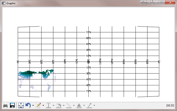I am not sure how to use the Image_Dimensions keyword, except to say I don't think it should be set to the dimensions of the image.

 

In any case, we don't have to use the Image_Dimensions and Image_Location keywords because we have longitude and latitude vectors that do the same thing. We can use those.

This leads us to another strange feature of the map projection software in IDL 8.1. Consider typing these commands instead of the commands above.

   w = Window(Dimension=[775, 425])
   imgObj = Image(scaledData, lon, lat, Limit=mapLimits, $
       Grid_Units=2, Map_Projection='Equirectangular', $
       Position=[0.05,0.05,0.95,0.80], RGB_Table=rgb, /Current)

This code results in the following error.

   % IMAGE: X and Y parameters must be evenly spaced

This is a strange error, because examination of the latitude and longitude vectors confirms that they couldn't be more evenly spaced!

   IDL> Print, lat
     90.000000       87.500000       85.000000       82.500000   ...
   IDL> Print, lon
     0.00000000       3.7500000       7.5000000       11.250000  ...

As it turns out, the error message is completely bogus. What is "wrong" with this command is that the map projection software doesn't like the latitude vector going from 90 to -90. It wants the latitude vector to go from -90 to 90! Reversing the latitude vector will produce the proper map projection.

   w = Window(Dimension=[775, 425])
   imgObj = Image(scaledData, lon, Reverse(lat), Limit=mapLimits, $
       Grid_Units=2, Map_Projection='Equirectangular', $
       Position=[0.05,0.05,0.95,0.80], RGB_Table=rgb, /Current)

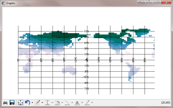The image is now properly located on the map projection, after taking care to orient the latitude and longitude vectors.

 

Changing Grid Properties

You notice in the figure above that the grid lines are fairly dense and are overpowering the image somewhat. This is probably an appropriate time to fix this by changing some of the properties of the grid. This is done by fetching the map projection object from the image object, and then fetching the grid object from the map projection object. In this case, we will change the grid spacing, the grid color and linestyle, and the position of the grid labels. It is not possible to change the position of the grid labels independently for the latitude and longitude labels. The code looks like this.

   map = imgObj.MapProjection
   grid = map.MapGrid
   grid.color = [120,120,120]
   grid.linestyle = 2
   grid.grid_longitude = 60
   grid.grid_latitude = 30
   grid.label_position = 0.95

It is also not possible (as far as I know) to label the longitudinal lines with values that go from 0 to 360.

Adding Continental Outlines

We can add continental outlines with the MapContinents function.

   c = MapContinents(Color=[70,70,70], /Current)

The image with the grid modifications and the continental outlines added can be seen in the figure below.

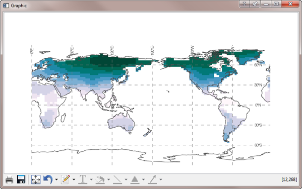The grid properties have been changed and continental outlines added to the map.

 

Adding a Colobar

The final step is to add a color bar to the graphic display. Adding a color bar is problematic in this case, because of the white color we are using to display the missing data. The color bar design does not allow color bars to have less than 256 colors. The only way around the problem is to use a fake data set to attach to the color bar. The code looks like this. Notice that we have to reload the colors without the white color being present and we have to hide the fake image so it doesn't appear on the display.

(Also note that the fake image has to use exactly the same parameters as the original image, for reasons I don't understand, or the graphic display already in the window will change in ways that make no sense to me. If you understand why this is so, please let me know.)

   cgLoadCT, 4, /Brewer, /Reverse, NColors=10
   TVLCT, rgb, /Get
   table = Congrid(rgb[0:9,*], 256, 3)
   levels = String(Round(cgScaleVector(Findgen(11), minValue, maxValue)), Format='(i0)')
   fakeImage = Image(scaledData, lon, Reverse(lat), Limit=mapLimits, $
       Grid_Units=2, Map_Projection='Equirectangular', $
       Position=[0.05,0.05,0.95,0.80], RGB_Table=table, /Current, /Hide)
   cb = Colorbar(Target=fakeImage, Tickname=levels, Major=11, /Border_On, $
      Position=[0.1, 0.88, 0.9, 0.93], TickLen=2.0, Minor=0)

There are several points to make about the Colorbar function. First, we have to override the actual values of the color bar and replace them with values from the data itself. We do this by creating the levels variable and passing it to the color bar with the Tickname keyword. I also find that I need to set the TickLen keyword to 2 in order to create defined boxes on the color bar. In direct graphics this keyword would be set to 1 to do the same thing.

The final result looks like the figure below. I do not know how, or even if it is possible, to put a border around the image, although one can make box axes for the grid. In the grid properties section above, add this line.

   grid.box_grid = 1

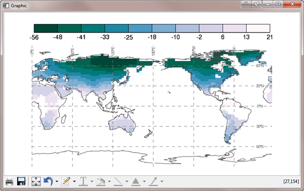The final image displayed on a map projection.

 

A program named ImgMap is available containing all the code above. It requires the imgmap.sav file to be found in the same directory as the source code to run correctly.

Easier with Coyote Graphics?

An map-image display like this is much easier to create with Coyote Graphics. To demonstrate how, I have created the same program, named Coyote_ImgMap using Coyote Graphics commands. To display this map in a resizeable graphics window, with the ability to create the same quality hardcopy output as function graphics, you would type this.

   cgWindow, 'Coyote_ImgMap'

You see the results below.

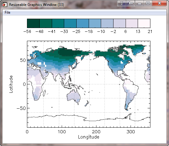The final image displayed on a map projection using Coyote Graphics commands.

 

Version of IDL used to prepare this article: IDL 8.1.